
Adversarial Mutual Information Learning for Network Embedding
Proceedings of the Twenty-Ninth International Joint Conference on Artificial Intelligence. Main track. Pages 3321-3327.
https://doi.org/10.24963/ijcai.2020/459
Keywords
- Multidisciplinary Topics and Applications: Web Analysis of Communities
- Machine Learning Applications: Networks
- Machine Learning: Adversarial Machine Learning
Abstract
Network embedding which is to learn a low dimensional representation of nodes in a network has been used in many network analysis tasks. Some network embedding methods, including those based on generative adversarial networks (GAN) (a promising deep learning technique), have been proposed recently. Existing GAN-based methods typically use GAN to learn a Gaussian distribution as a priori for network embedding. However, this strategy makes it difficult to distinguish the node representation from Gaussian distribution. Moreover, it does not make full use of the essential advantage of GAN (that is to adversarially learn the representation mechanism rather than the representation itself), leading to compromised performance of the method. To address this problem, we propose to use the adversarial idea on the representation mechanism, i.e. on the encoding mechanism under the framework of autoencoder. Specifically, we use the mutual information between node attributes and embedding as a reasonable alternative of this encoding mechanism (which is much easier to track). Additionally, we introduce another mapping mechanism (which is based on GAN) as a competitor into the adversarial learning system. A range of empirical results demonstrate the effectiveness of the proposed approach.
- [Cao et al., 2015] Shaosheng Cao, Wei Lu, and Qiongkai Xu. Grarep: Learning graph representations with global structural information. In Proceedings of the 24th ACM in- ternational on conference on information and knowledge management, pages 891-900, Melbourne, Australia, Oc- tober 2015. ACM.
- [Dai et al., 2018] Quanyu Dai, Qiang Li, Jian Tang, and Dan Wang. Adversarial network embedding. In Thirty-Second AAAI Conference on Artificial Intelligence, pages 2167- 2174, New Orleans, Louisiana, USA, February 2018. AAAI.
- [Ding et al., 2018] Ming Ding, Jie Tang, and Jie Zhang. Semi-supervised learning on graphs with generative adver- sarial nets. In Proceedings of the 27th ACM International Conference on Information and Knowledge Management, pages 913-922, Torino, Italy, October 2018. ACM.
- [Donahue et al., 2017] Jeff Donahue, Philipp Krähenbühl, and Trevor Darrell. Adversarial feature learning. In Inter- national Conference on Learning Representations, 2017.
- [Goodfellow et al., 2014] Ian Goodfellow, Jean Pouget- Abadie, Mehdi Mirza, Bing Xu, David Warde-Farley, Sherjil Ozair, Aaron Courville, and Yoshua Bengio. Gen- erative adversarial nets. In Advances in neural information processing systems, pages 2672-2680, Montreal, Quebec, Canada, 2014. MIT Press.
- [Grover and Leskovec, 2016] Aditya Grover and Jure Leskovec. Node2vec: Scalable feature learning for networks. In Proceedings of the 22nd ACM SIGKDD international conference on Knowledge discovery and data mining, pages 855-864, San Francisco, California, USA, August 2016. ACM.
- [Hjelm et al., 2019] R Devon Hjelm, Alex Fedorov, Samuel Lavoie-Marchildon, Karan Grewal, Phil Bachman, Adam Trischler, and Yoshua Bengio. Learning deep representa- tions by mutual information estimation and maximization. In International Conference on Learning Representations, 2019.
- [Huang et al., 2017] Xiao Huang, Jundong Li, and Xia Hu. Accelerated attributed network embedding. In Proceed- ings of the 2017 SIAM international conference on data mining, pages 633-641, Houston, Texas, USA, April 2017. IEEE.
- [Jin et al., 2019a] Di Jin, Bingyi Li, Pengfei Jiao, Dongxiao He, and Weixiong Zhang. Network-specific variational auto-encoder for embedding in attribute networks. In Pro- ceedings of the Twenty-Eighth International Joint Con- ference on Artificial Intelligence, IJCAI-19, pages 2663- 2669. International Joint Conferences on Artificial Intelli- gence Organization, 7 2019. IJCAI
- [Jin et al., 2019b] Di Jin, Ziyang Liu, Weihao Li, Dongxiao He, and Weixiong Zhang. Graph convolutional networks meet markov random fields: Semi-supervised community detection in attribute networks. In Proceedings of the AAAI Conference on Artificial Intelligence, volume 33, pages 152-159, 2019.
- [Kipf and Welling, 2016] Thomas N Kipf and Max Welling. Variational graph auto-encoders. arXiv preprint arXiv:1611.07308, 2016.
- [Kipf and Welling, 2017] Thomas Kipf and Max Welling. Semi-supervised classification with graph convolutional networks. In International Conference on Learning Rep- resentations, 2017.
- [Liao et al., 2018] Lizi Liao, Xiangnan He, Hanwang Zhang, and Tat-Seng Chua. Attributed social network embedding. IEEE Transactions on Knowledge and Data Engineering, 30(12):2257-2270, 2018.
- [Liu et al., 2012] Haifeng Liu, Zhaohui Wu, Xuelong Li, Deng Cai, and Thomas S Huang. Constrained nonnega- tive matrix factorization for image representation. IEEE Transactions on Pattern Analysis and Machine Intelli- gence, 34(7):1299-1311, 2012.
- [Maaten and Hinton, 2008] Laurens van der Maaten and Ge- offrey Hinton. Visualizing data using t-sne. Journal of machine learning research, 9(Nov):2579-2605, 2008.
- [Pan et al., 2016] Shirui Pan, Jia Wu, Xingquan Zhu, Chengqi Zhang, and Yang Wang. Tri-party deep network representation. Network, 11(9):12, 2016. IJCAI
- [Pan et al., 2018] Shirui Pan, Ruiqi Hu, Guodong Long, Jing Jiang, Lina Yao, and Chengqi Zhang. Adversarially regu- larized graph autoencoder for graph embedding. In Inter- national Joint Conference on Artificial Intelligence, pages 2609-2615, 2018. IJCAI
- [Perozzi et al., 2014] Bryan Perozzi, Rami Alrfou, and Steven Skiena. Deepwalk: online learning of social repre- sentations. In Proceedings of the 20th ACM SIGKDD in- ternational conference on Knowledge discovery and data mining, pages 701-710, New York, USA, August 2014. ACM.
- [Tang et al., 2015] Jian Tang, Meng Qu, Mingzhe Wang, Ming Zhang, Jun Yan, and Qiaozhu Mei. Line: Large- scale information network embedding. In Proceedings of the 24th international conference on world wide web, pages 1067-1077, Florence, Italy, May 2015. ACM.
- [Veličković et al., 2019] Petar Veličković, William Fedus, William L Hamilton, Pietro Liò, Yoshua Bengio, and R Devon Hjelm. Deep graph infomax. In International Conference on Learning Representations, 2019.
- [Wang et al., 2016] Daixin Wang, Peng Cui, and Wenwu Zhu. Structural deep network embedding. In Proceed- ings of the 22nd ACM SIGKDD international conference on Knowledge discovery and data mining, pages 1225- 1234. ACM, 2016.
- [Yu et al., 2018] Wenchao Yu, Cheng Zheng, Wei Cheng, Charu C Aggarwal, Dongjin Song, Bo Zong, Haifeng Chen, and Wei Wang. Learning deep network representa- tions with adversarially regularized autoencoders. In Pro- ceedings of the 24th ACM SIGKDD International Con- ference on Knowledge Discovery & Data Mining, pages 2663-2671, London, United Kingdom, August 2018. ACM.
References were extracted automatically from the PDF and may contain errors.
Full text extracted automatically from the PDF; figures, tables and equations may differ. The PDF is the version of record.
1 Introduction
Network embedding aims to represent the nodes of a network by low-dimensional vectors, and then use this lowdimensional representation for network analysis tasks such as link predictions, node classification, network visualization, user recommendation and community detection [Wang et al., 2016], MRFasGCN [Jin et al., 2019b].
Most of the existing network embedding algorithms use information of network topologies, including DeepWalk [Perozzi et al., 2014], LINE [Tang et al., 2015], GraRep [Cao et al., 2015] and Node2Vec [Grover and Leskovec, 2016]. Rich information of node attributes consistent with information of network topologies has also been explored in network embedding in recent years, including TriDNR [Pan et al., 2016], SNE [Liao et al., 2018] and NetVAE [Jin et al., 2019a].
∗Corresponding author.
Particularly, Generative Adversarial Networks (GAN) [Goodfellow et al., 2014], originally proposed for generating images, has been extended to network embedding recently. For example, ANE [Dai et al., 2018] leverages the adversarial learning principle to regularize the representation learning by matching the posterior distribution of the latent representations to given priors (e.g. Gaussian distribution). ARGA [Pan et al., 2018] encodes the topological structure and node contents in a graph to a compact representation, where a decoder is trained to reconstruct the graph structure. The latent representation is then enforced to match a prior distribution via adversarial training. NetRA [Yu et al., 2018] proposes to learn the network representations with adversarially regularized autoencoders and learn the smoothly regularized vertex representations through jointly considering both locality-preserving and global reconstruction constraints. In GraphSGAN [Ding et al., 2018], a novel approach for semi-supervised learning on graphs (where generator implicitly generates fake samples in low-density areas between subgraphs and classifier implicitly), takes the density property of subgraph into consideration.
It is worth noting that these existing methods typically apply the adversarial learning strategy on the representation of nodes, e.g. matching the distribution of node representation to an arbitrary prior (such as Gaussian distribution in most cases). However, this strategy makes it difficult to distinguish the node representation from Gaussian noise, since it requires the representation to obey the Gaussian distribution, which roughly equals adding a Gaussian regular term to the representation. While this is reasonable to some extent, it does not make full use of the essential advantage of adversarial learning. We believe it is better to apply the adversarial learning strategy on the representation mechanism that projects data onto latent space (to make the system robust and effective) rather than on the representation itself (which simply requires the representation distribution to follow priors).
Based on this idea, we proposed a novel adversarial learning approach for network embedding under the framework of autoencoder. The core of this model is adversarial learning on the representation mechanism, i.e. on the encoding mechanism in encoder, which however, is still difficult to operate. Since it is often believed that the mapping mechanism can be expressed approximately by the mutual information of the input and output of the mapping [Hjelm et al., 2019], which is much easier to address, we use this mutual information to measure the quality of the mapping mechanism. Additionally, we introduce another mapping mechanism as a competitor into the adversarial learning system, and let the competitor competes with the encoder in their mapping mechanisms. Competition in this game motivates both the competitor and the encoder to improve their mapping methods, resulting in an effective encoder with competitive representation mechanism. Considering the fact that basic GAN model with a generator and a discriminator can capture semantic variation in data distribution through its latent space [Donahue et al., 2017], we use the basic GAN generator as the competitor of our adversarial learning model. Then, the discriminator is trained to discriminate the mapping mechanism of the encoder from that of the competitor.
2 Preliminaries
We first give the notations and define the problem. We then introduce Generative adversarial networks (GAN) which is the base of our approach.
2.1 Notations and the Problem
Consider an undirected, unweighted and attributed network N = (V, E,X) with n nodes V = {v1, v2, . . . , vn}, a set of edges E = {eij} ⊆ V × V , and a set of node attribute X ∈ Rn×T , where T represents the number of attributes of each node. The topological structure of N is represented by an adjacency matrix A = [aij ] ∈ Rn×n , where aij = 1 if nodes vi and vj are connected, or aij = 0 otherwise. Attribute xi ∈ X specifies the features or properties of node vi. The objective of network embedding is to cast each of the n nodes in the network to a vector hi ∈ Rk (where k ≪ n).
2.2 Generative Adversarial Networks
Generative adversarial networks (GAN) are inspired by the two-player game in game theory. The two players in the GAN model are a generator G and a discriminator D. The goal of the generator is to generate samples that are as similar to the real training examples as possible. This is done by learning the underlying distribution of the real data. As real data are often noisy, a variable of noise z is typically introduced into the GAN model. The goal of the discriminator, on the other hand, is to distinguish synthetic samples (generated by the generator) from the real ones as accurately as possible. In particular, discriminator is a two-class classifier that estimates the probability of a sample being synthetic or real. In the iterative process of training, with one part (generator or discriminator) being fixed, the parameters of the other part are updated. In the process of competitive confrontation between the generator and discriminator, both parties try to optimize their own objectives until a dynamic equilibrium is established. At equilibrium, the resulting generative model from generator captures the latent distribution of the training data so that the discriminator can no longer accurately separate the synthetic samples from the real ones with an accuracy rate above 50%. The above process can be expressed as:
where the first expectation is the loss of discriminator for real training samples and the second the loss of discriminator for synthetic samples (generated by the generator).
3 The Approach
We first give a brief overview of the proposed method, and then introduce three elements of the model in detail. At last, we give the proposed Adversarial Mutual Information Learning approach (AMIL).
3.1 Overview
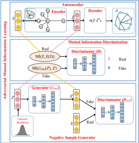
To adversarially learn an effective embedding mechanism, we leverage mutual information to express the mapping mechanism from data space to latent space (or vice versa), and introduce a basic GAN generator into the whole adversarial learning model as a competitor. The structure of our adversarial mutual information learning approach is illustrated in Figure 1. It includes three elements: an autoencoder, a negative sample generator (which is the introduced competitor) and a mutual information discriminator.
In the autoencoder, the encoder (E) transforms the node attributes (X) into the embedding (Z = E(X)) utilizing the network topology, and the decoder reconstructs the topology using this embedding. The negative sample generator includes a generator (GNSG) and the attribute discriminator (DNSG) (with respect to the mutual information discriminator D). It is a basic GAN model where the latent space Z ′ of such model can capture semantic variation in the real data, i.e., the node attribute X. The mutual information discriminator (D) identifies the mapping mechanism of the encoder from that of the negative sample generator with the help of the mutual information. In our AMIL model, we not only train an encoder but also train a generator. The encoder is trained with dual objectives: a traditional reconstruction error criterion of autoencoder and an adversarial training criterion from the mutual information discriminator (D). The training of generator (GNSG) in negative sample generator also has dual objectives: an adversarial training criterion from the mutual information discriminator (D) and an adversarial training criterion of negative sample generator from the attribute discriminator (DNSG).
It is worth noting that the model can be also taken as framework that naturally combines node attributes (X) and topological structure (A) into the embedding representation (Z). The decoder of autoencoder feeds back a reconstruction error criterion (with topological information) to the encoder. Meanwhile, the mutual information discriminator (D) feeds back an adversarial training criterion (with attributes information) to the encoder. Then the encoder uses the two types of feedbacks to update its weight parameters. The above three steps are performed iteratively, and then a compact representation containing both topology and attributes is obtained.
3.2 The Autoencoder
We use the autoencoder framework similar to graph autoencoder [Kipf and Welling, 2016]. First, we use the graph convolutional networks (GCN) [Kipf and Welling, 2017] as the encoder to extract the embedding of nodes. In this paper, we use the classic two-layer GCN. Given the adjacency matrix A and attribute matrix X of a network, the model is constructed as
with each convolutional layer expressed by
Here ˜ A = A + I (where I is the identity matrix) and ˜Dii = ∑j ˜ Aij. W (l) denotes the weight parameters to be trained and Z (l) the output embedding in this layer. φ is an activation function such as Relu(t) = max(0, t) used in the first layer and Linear(t) = t used in the second layer. In the decoder, we reconstruct the network topology using the embedding derived from the encoder. Given the embedding Z = Z (2) , using the inner product method the reconstructed graph ˆ A can be presented as
We then use the cross entropy to define the loss as
3.3 Negative Sample Generator
The negative sample generator, which is a basic GAN, can play the role of a competitor in the whole adversarial learning system, if the following two conditions are met. First, it is an effective mapping mechanism. Second, it is a multi-layer perceptron. Since classical GAN is indeed a multi-layer perceptron, we only need to show the first condition is also satisfied (to show the negative sample generator can be a competitor). It is well known that a basic GAN learns a generator mapping from arbitrarily latent distribution to the data. Recent work also showed that the latent space of such generator captures sematic variation in real data [Donahue et al., 2017]. This may indicate that GAN is indeed an effective mapping mechanism (satisfying the first condition). Thus, the negative sample generator can be a competitor.
The negative sample generator includes two parts: a generator (GNSG) and a discriminator (DNSG). The generator (GNSG) uses a three-layer fully-connected network which takes a Gaussian noise Z ′ as input and generates the attribute of the nodes (X′ = GNSG(Z ′ )). The generator (GNSG) generates fake node attributes X′ based on latent variables Z ′ , to deceive the discriminator (DNSG). The discriminator (DNSG) attempts to identify the real attribute from the fake one. By interactive training, the generated attributes of the nodes can look more like the real data.
Here the loss of the generator (GNSG) is defined as
where z′ is a sample that satisfies the simple Gaussian distribution pz′ (z′ ), GNSG(z′ ) and DNSG(·) indicate the generator and discriminator explained above.
The loss of the discriminator (DNSG) is defined as
where pdata(x) is the sample distribution of x.
The training objective of the negative sample generator can be defined as a minimax objective
Compared with the simple generator, which does not have a discriminator and thus is not a GAN model, our negative sample generator has the following advantages. First, it can produce node attribute information which is more similar to the real one in the data, thanks to the adversarial learning of the generator and discriminator in the GAN model. Second, the discriminator (DNSG) in the GAN model can make the generated node attributes (X′ ) not deviate much from the given ones (X). This will limit the solution space for model training and parameter tuning.
3.4 The Mutual Information Discriminator
The core of our model is to apply adversarial learning strategy on the representation mechanism rather than on the representation itself, so as to learn an effective encoding mechanism. The encoding mechanism can be regarded as a representation learning function as well as the relationship between its input and output variable. Mutual information can represent the relationship between two variables. Recent research showed that the encoding mechanism can be expressed approximately by the mutual information of the input and output of the encoder [Hjelm et al., 2019], which is much easier to track. Then, we use the mutual information between the input variable (node attributes X) and the output variable (node embedding Z) of the encoder to express the encoding mechanism. The mutual information between node attributes and the node representation of the encoder, denoted by (MI(X,Z)), can track the quality of the encoding process. That is, when the mutual information between node attributes and the representation is larger, this representation will be more representative of the nodes in the network. While the mutual information (MI(X, Z)) can be defined in many ways, here we take the concatenation of X and Z as an effective relaxation and approximation (since it can well describe the mapping between X and Z and is the simplest way for learning efficiently).
In specific, we use the mutual information of the nodes representation (Z) (generated by the encoder) and the attribute information (X) together as the positive sample mutual information (MI(X,Z)). On the other hand, we use the mutual information of the input (Z ′ ) and output (GNSG(Z ′ )) of the negative sample generator as the negative sample mutual information (MI(X′ ,Z ′ )). Once we get the mutual information sampled from the encoder and the negative sample generator, we send the positive samples and the negative samples to the mutual information discriminator (D). The discriminator attempts to discriminate the negative samples generated by the generator as 0, and the positive samples generated by the encoder as 1. Then, we can define the loss of the discrimination (D) as
3.5 Adversarial Mutual Information Learning
In this section, we will give the whole AMIL model. We use the mutual information of the input (X) and the output (Z = E(X)) of the encoder as a positive sample mutual information (with the help of decoder which reconstructs the network topology). Therefore, the loss of the encoder is divided into two parts: one part is the loss of the reconstructed topology, expressed as Eq. (5). Another part is the loss from adversarial training criterion, i.e., the loss that the mutual information discriminator (D) is deceived by the positive sample mutual information (MI(X,Z)) and thus takes it as a negative one.
Then, we can define the overall loss of the encoder as
Meanwhile, we use the mutual information of the input (Z ′ ) and the output (X′ = GNSG(Z ′ )) of the negative sample generator as a negative sample mutual information. Then, the loss of the generator (GNSG) is divided into two parts: One part is the loss from negative sample generator, expressed as Eq. (6). The other part is the loss from the mutual information discriminator (D), i.e., the loss that D is deceived by the negative sample mutual information and thus takes it as the positive one. We define the loss from the mutual information discriminator as
Then, we can define the overall loss of the generator (GNSG) as
The mutual information discriminator (D) attempts to identify the mutual information of node attributes and embedding from either the encoder (positive sample) or the generator GNSG (negative sample). Therefore, the AMIL training objective is defined as a minimax objective
where
We optimize the minimax objective (15) using the same alternating gradient-based optimization as [Donahue et al., 2017]. Our model jointly trains an encoder (E) and a generator (GNSG). At the global optimum of the whole adversarial learning, encoder (E) and generator (GNSG) are each other's inverse.
4 Experiments
We first give the experimental setup, and then compare the new approach AMIL with some state-of-the-art methods on three network analysis tasks, i.e., node classification, node clustering and network visualization. Next, we perform a comparative experiment with a simple generator or with a GAN generator, i.e., with or without discriminator DNSG. We finally give the parameter analysis.
4.1 Experimental Setup
Datasets. Seven publicly available datasets 1 with varying sizes and characteristics are used, which are representative of two types of networks: webpage networks (Cornell, Texas, Washington and Wisconsin from the WebKB dataset) and document networks (Citeseer, Cora and Pubmed). The detailed information of the seven datasets are summarized in Table 1.
1 https://linqs.soe.ucsc.edu/data
| Datasets | Cornell | Texas | Waton | Wisin | Cora | Cite | Pubmed |
|---|---|---|---|---|---|---|---|
| Nodes | 195 | 183 | 217 | 262 | 2,708 | 3,312 | 19,717 |
| Edges | 304 | 328 | 446 | 530 | 5,429 | 4,732 | 44,338 |
| Classes | 5 | 5 | 5 | 5 | 7 | 6 | 3 |
| Attributes | 1,703 | 1,703 | 1,703 | 1,703 | 1,433 | 3,703 | 500 |
Baseline Methods. We compared our approach AMIL with ten embedding methods: (1) the methods using network topology: DeepWalk [Perozzi et al., 2014], Node2Vec [Grover and Leskovec, 2016], LINE [Tang et al., 2015] and GraRep [Cao et al., 2015], and (2) the methods using both topological and semantic information: TriDNR [Pan et al., 2016], AANE [Huang et al., 2017], SNE [Liao et al., 2018], VGAE [Kipf and Welling, 2016], ARVGE [Pan et al., 2018] and DGI [Veliˇckovi´c et al., 2019]. Especially, ARVGE [Pan et al., 2018] is a state-of-the-art network embedding method based on GAN.
Parameter Settings. The final embedding dimension is often set to power of 2. To ensure fairness, we uniformly set it to 64 for all the methods on all the datasets. The parameters of the methods compared were set as what were used by their authors. For DeepWalk, we set the walk length as 40 and window size as 5. For Node2Vec, we set the walk length as 80 and window size as 10. For LINE, we set the number of negative samples used in negative sampling as 5 and the starting value of the learning rate as 0.025. For GraRep, we set the maximum matrix transition step as 5. In our approach AMIL, for the encoder, we use the classic two-layer GCN, which has 128 units in the first layer and 64 units in the second layer. For the discriminators (DNSG and D), we use three layers of fully connected neural network. In specific, 512 units for first two layers and 1 unit for last layer. We use ReLU(·) as the activation function in the first two layers, and use Sigmoid(·) in the last layer. We use the pytorch deep learning tools to learn the model with a learning rate of 0.001.
Evaluation Metrics. In node classification, we use accuracy (AC) as the metric to evaluate the performance of all methods. For node clustering (a.k.a. community detection), besides accuracy [Liu et al., 2012], we also use normalized mutual information (NMI) [Liu et al., 2012] as an additional accuracy metric since NMI has been more often used in node clustering.
4.2 Node Classification
In node classification, our goal is to classify each node into one of the multiple labels. After getting the network embedding, we adopt the LibSVM and LibLINEAR software packages in Weka to classify these nodes with ground-truth. For each network, we used 10-fold cross-validation and accuracy (AC) as the metric to evaluate the performance of all methods.
| Packages | Methods | Cornell | Texas | Waton | Wisin | Cora | Cite | Pubmed |
|---|---|---|---|---|---|---|---|---|
| LibSVM | DeepWalk | 38.97 | 49.18 | 55.30 | 49.24 | 82.57 | 52.52 | 78.79 |
| Node2Vec | 35.90 | 50.27 | 47.47 | 46.56 | 79.98 | 61.63 | 80.30 | |
| LINE | 43.59 | 68.85 | 59.91 | 54.58 | 30.20 | 41.07 | 75.47 | |
| GraRep | 53.33 | 62.68 | 52.07 | 59.16 | 73.41 | 54.28 | 80.64 | |
| AANE | 51.80 | 56.28 | 64.06 | 43.13 | 30.20 | 24.70 | 78.63 | |
| TriDNR | 37.95 | 48.09 | 47.01 | 40.46 | 43.27 | 54.47 | 79.07 | |
| SNE | 48.21 | 57.92 | 54.38 | 59.54 | 49.00 | 44.74 | 78.37 | |
| VGAE | 45.13 | 55.00 | 54.38 | 53.82 | 81.05 | 65.97 | 83.42 | |
| ARVGE | 42.56 | 56.28 | 58.99 | 49.26 | 80.42 | 65.10 | 80.64 | |
| DGI | 42.56 | 56.28 | 47.47 | 45.42 | 80.21 | 70.07 | 74.57 | |
| AMIL | 53.58 | 68.92 | 65.76 | 59.70 | 83.60 | 70.99 | 80.81(2) | |
| DeepWalk | 38.46 | 48.09 | 53.92 | 49.62 | 82.04 | 48.42 | 78.36 | |
| Node2Vec | 37.95 | 50.27 | 45.62 | 46.95 | 80.79 | 52.44 | 80.08 | |
| LINE | 44.10 | 53.39 | 56.22 | 54.96 | 50.25 | 40.56 | 74.92 | |
| GraRep | 53.33 | 59.40 | 51.15 | 60.31 | 79.83 | 53.61 | 80.37 | |
| AANE | 41.54 | 53.01 | 61.75 | 38.93 | 27.03 | 22.24 | 77.99 | |
| LibLINEAR | TriDNR | 34.87 | 42.08 | 43.32 | 41.60 | 53.39 | 52.91 | 78.40 |
| SNE | 45.64 | 59.02 | 55.76 | 59.92 | 54.46 | 44.35 | 77.20 | |
| VGAE | 45.64 | 51.91 | 54.84 | 54.49 | 79.13 | 69.25 | 83.81 | |
| ARVGE | 41.54 | 59.02 | 60.37 | 56.11 | 81.24 | 66.71 | 80.59 | |
| DGI | 43.08 | 56.28 | 55.31 | 48.86 | 84.71 | 70.85 | 78.11 | |
| AMIL | 54.15 | 59.73 | 62.53 | 61.16 | 81.46(3) | 71.36 | 80.98(2) |
The results are shown in Table 2. As shown, our method AMIL performs the best on 6 of the 7 networks in LibSVM and 5 of the 7 networks in LibLINEAR. On average, AMIL outperformed the best baseline method (i.e. ARVGE) in node classification by 13.46% using LibSVM and by 10.08% using LibLINEAR. In particular, AMIL performs better than the other GAN-based method (i.e. ARVGE) on all networks, an obvious improvement.
4.3 Node Clustering
In node clustering, we aim to assign distinct cluster to each node. After having the embedding of all the algorithms, we applied k-means algorithm to the resulting embedding of nodes to cluster them into classes (as done by the existing works). Here, we use both the AC and NMI as the performance metrics as discussed above.
The results are shown in Table 3. As shown, our method AMIL performs the best on 6 of the 7 networks in terms of both AC and NMI. On the remaining networks where our AMIL does not perform the best, it still has the second best results. On average, AMIL outperformed the best baseline method (i.e. DGI) in node clustering by 10.45% in terms of AC and 18.91% in terms of NMI. In particular, AMIL performs better than the other GAN-based method (i.e. ARVGE) on all the datasets. This further validate the effectiveness of the new approach.
4.4 Visualization
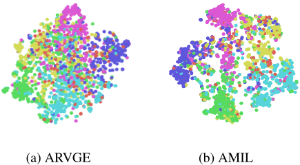
To further illustrate that the embedding from our method is an accurate representation, we also visualize the embedding of some representative network embedding methods (i.e. ARVGE [Pan et al., 2018] and our AMIL) in the Citeseer dataset as an example. We use the t-SNE [Maaten and Hinton, 2008] tool to reduce the result of embedding representation to two dimensions and draw a color for each categorical label. The result is given in Figure 2.
As shown in Figure 2 (a), the representations derived from ARVGE are also tightly interweaved, and thus it is still not easy to distinguish them. In contrast, our embedding results in Figure 2 (b) show that the nodes are divided into different categories more clearly. That is, nodes with the same color are roughly gathered together. This further demonstrate that our model can obtain a better representation.
| Metrics (%) | Methods | Cornell | Texas | Waton | Wisin | Cora | Cite | Pubmed |
|---|---|---|---|---|---|---|---|---|
| AC | DeepWalk | 36.05 | 46.72 | 40.76 | 38.76 | 45.61 | 36.21 | 64.84 |
| Node2Vec | 33.85 | 47.54 | 37.33 | 49.62 | 56.30 | 40.76 | 65.56 | |
| LINE | 39.49 | 53.38 | 52.68 | 45.43 | 30.72 | 25.01 | 43.11 | |
| GraRep | 31.79 | 36.72 | 31.36 | 33.24 | 48.29 | 31.20 | 54.43 | |
| AANE | 37.28 | 30.49 | 41.57 | 30.53 | 18.51 | 21.76 | 34.55 | |
| TriDNR | 38.21 | 47.54 | 43.59 | 43.70 | 31.56 | 34.44 | 59.29 | |
| SNE | 41.08 | 41.53 | 48.80 | 55.30 | 39.44 | 31.17 | 65.13 | |
| VGAE | 36.72 | 48.35 | 43.73 | 43.28 | 57.06 | 53.46 | 58.64 | |
| ARVGE | 38.21 | 41.48 | 43.66 | 42.81 | 64.08 | 43.50 | 58.76 | |
| DGI | 38.46 | 51.91 | 48.85 | 45.80 | 63.51 | 67.54 | 64.07 | |
| AMIL | 44.62 | 57.92 | 54.38 | 55.34 | 72.89 | 64.44(2) | 66.12 | |
| DeepWalk | 7.06 | 6.16 | 5.66 | 7.65 | 31.51 | 10.58 | 25.55 | |
| Node2Vec | 6.65 | 4.49 | 2.94 | 7.86 | 42.02 | 12.99 | 25.02 | |
| LINE | 9.27 | 18.16 | 18.95 | 9.39 | 10.13 | 5.62 | 7.17 | |
| GraRep | 8.80 | 12.43 | 5.18 | 8.02 | 35.46 | 9.61 | 17.76 | |
| NMI | AANE | 9.55 | 3.52 | 13.19 | 2.86 | 0.40 | 1.19 | 0.01 |
| TriDNR | 7.20 | 4.32 | 8.10 | 6.60 | 12.19 | 9.59 | 19.28 | |
| SNE | 11.11 | 12.63 | 17.43 | 18.94 | 16.28 | 7.31 | 25.61 | |
| VGAE | 7.77 | 8.52 | 9.03 | 9.31 | 42.92 | 27.93 | 17.83 | |
| ARVGE | 10.26 | 7.28 | 12.60 | 11.92 | 44.95 | 22.72 | 18.40 | |
| DGI | 12.52 | 13.98 | 15.64 | 13.69 | 49.76 | 42.74 | 26.64 | |
| AMIL | 14.81 | 18.45 | 20.71 | 19.98 | 54.88 | 37.71(2) | 28.03 |
4.5 Comparative Test with Simple Generator or with a GAN Generator
In this section, we want to evaluate whether our negative sample generator, which is a GAN generator, is better than a simple generator, which does not have a discriminator. In other words, we want to evaluate the impact of the attribute discriminator (DNSG). Specifically, we use the same clustering method as in Section 4.3 to obtain experimental results with and without the discriminator (DNSG). The model with the discriminator (DNSG) is our AIML, and the method without the discriminator (DNSG) is called AIML ND. Similarly, we use both the AC and NMI as the performance metrics as discussed earlier.
The results are shown in Table 4. As shown, our method AMIL performs better than AIML ND on the 7 networks in AC and NMI. On average, AMIL outperformed AIML ND in node clustering by 6.21% in terms of AC and 17.29% in terms of NMI. This further shows that the discriminator (DNSG) can help the generator generate more effective negative sample mutual information, resulting in more robust embedding.
| Metrics (%) | Methods | Cornell | Texas | Waton | Wisin | Cora | Cite | Pubmed |
|---|---|---|---|---|---|---|---|---|
| AC | AIML ND | 42.56 | 52.46 | 53.46 | 48.47 | 71.01 | 59.15 | 65.64 |
| AMIL | 44.62 | 57.92 | 54.38 | 55.34 | 72.89 | 64.44 | 66.12 | |
| NMI | AIML ND AMIL | 12.01 | 12.90 | 19.03 | 16.41 | 53.49 | 32.69 | 26.41 |
| 14.81 | 18.45 | 20.71 | 19.98 | 54.88 | 37.71 | 28.03 |
4.6 Parameter Analysis
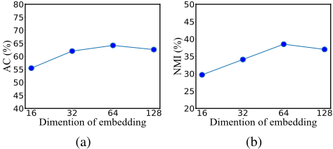
In this section, we analyze the effect of the embedding dimension on the model's performance. We select the embedding dimensions of 16, 32, 64 and 128. The experimental results are shown in Figure 3. Figure 3 (a) shows the result of network embedding with different dimensions in terms of AC (still on the node clustering task in Citeseer), and (b) shows that in terms of NMI. As shown, in terms of AC, the algorithm's performance is relatively stable with the change of the dimensions of network embedding, while it has some small fluctuations in terms of NMI. This validates that the algorithm is robust to the dimensions of network embedding.
5 Conclusions
To better utilize the essential advantage of GAN on network embedding, we propose a new approach of adversarial mutual information learning for network embedding (AMIL), which uses adversarial learning strategy on the representation mechanism rather than on embedding results. We use mutual information to express a mapping mechanism of an encoder (or generator) approximately, which makes the discriminator really work. In addition, another mapping function, i.e. negative sample generator, is introduced to the adversarial learning system as a competitor. The method proposed is evaluated on some real datasets with different scales. Experimental results show that the new method significantly outperforms the state-of-the-art methods including another GANbased method.
Acknowledgments
This work was supported in part by the Natural Science Foundation of China (61876128, 61772361, 61972442), the George Washington University Facilitating Fund (UFF) FY21, and the NSF under grants III-1526499, III-1763325, III-1909323, and CNS-1930941.
@inproceedings{ijcai2020p459,
  title     = {Adversarial Mutual Information Learning for Network Embedding},
  author    = {He, Dongxiao and Zhai, Lu and Li, Zhigang and Jin, Di and Yang, Liang and Huang, Yuxiao and Yu, Philip S.},
  booktitle = {Proceedings of the Twenty-Ninth International Joint Conference on
               Artificial Intelligence, {IJCAI-20}},
  publisher = {International Joint Conferences on Artificial Intelligence Organization},
  editor    = {Christian Bessiere},
  pages     = {3321--3327},
  year      = {2020},
  month     = {7},
  note      = {Main track},
  doi       = {10.24963/ijcai.2020/459},
  url       = {https://doi.org/10.24963/ijcai.2020/459},
}
TY - CPAPER TI - Adversarial Mutual Information Learning for Network Embedding AU - He, Dongxiao AU - Zhai, Lu AU - Li, Zhigang AU - Jin, Di AU - Yang, Liang AU - Huang, Yuxiao AU - Yu, Philip S. T2 - Proceedings of the Twenty-Ninth International Joint Conference on Artificial Intelligence, IJCAI-20 PB - International Joint Conferences on Artificial Intelligence Organization PY - 2020 SP - 3321 EP - 3327 DO - 10.24963/ijcai.2020/459 UR - https://doi.org/10.24963/ijcai.2020/459 ER -Copied
Machine-readable versions of this paper, for tools and AI agents:





