
Inverse Reinforcement Learning for Team Sports: Valuing Actions and Players
Proceedings of the Twenty-Ninth International Joint Conference on Artificial Intelligence. Main track. Pages 3356-3363.
https://doi.org/10.24963/ijcai.2020/464
Keywords
- Agent-based and Multi-agent Systems: Other
- Machine Learning Applications: Applications of Reinforcement Learning
- Machine Learning: Reinforcement Learning
Abstract
A major task of sports analytics is to rank players based on the impact of their actions. Recent methods have applied reinforcement learning (RL) to assess the value of actions from a learned action value or Q-function. A fundamental challenge for estimating action values is that explicit reward signals (goals) are very sparse in many team sports, such as ice hockey and soccer. This paper combines Q-function learning with inverse reinforcement learning (IRL) to provide a novel player ranking method. We treat professional play as expert demonstrations for learning an implicit reward function. Our method alternates single-agent IRL to learn a reward function for multiple agents; we provide a theoretical justification for this procedure. Knowledge transfer is used to combine learned rewards and observed rewards from goals. Empirical evaluation, based on 4.5M play-by-play events in the National Hockey League (NHL), indicates that player ranking using the learned rewards achieves high correlations with standard success measures and temporal consistency throughout a season.
- [Albert et al., 2017] Jim Albert, Mark E Glickman, Tim B Swartz, and Ruud H Koning. Handbook of Statistical Methods and Analyses in Sports. 2017.
- [Decroos et al., 2018] Tom Decroos, Lotte Bransen, Jan Van Haaren, and Jesse Davis. Actions speak louder than goals: Valuing player actions in soccer. arXiv preprint arXiv:1802.07127v1, 2018.
- [Decroos et al., 2019] Tom Decroos, Lotte Bransen, Jan Van Haaren, and Jesse Davis. Actions speak louder than goals: Valuing player actions in soccer. In Proceedings of the 25th International Conference on Knowledge Discovery & Data Mining (KDD-19), pages 1851-1861, 2019.
- [Gerstenberg et al., 2014] Tobias Gerstenberg, Tomer Ull- man, Max Kleiman-Weiner, David Lagnado, and Josh Tenenbaum. Wins above replacement: Responsibility at- tributions as counterfactual replacements. In Proceedings of the Annual Meeting of the Cognitive Science Society, volume 36, 2014.
- [Gretton et al., 2012] Arthur Gretton, Karsten M Borgwardt, Malte J Rasch, Bernhard Schölkopf, and Alexander Smola. A kernel two-sample test. Journal of Machine Learning Research, 13(Mar):723-773, 2012.
- [Jaynes, 1957] Edwin T Jaynes. Information theory and sta- tistical mechanics. Physical review, 106(4):620, 1957.
- [Littman, 1994] Michael L Littman. Markov games as a framework for multi-agent reinforcement learning. In Pro- ceedings of the 11st International Conference on Machine learning (ICML-94), volume 157, pages 157-163. 1994.
- [Liu and Schulte, 2018] Guiliang Liu and Oliver Schulte. Deep reinforcement learning in ice hockey for context- aware player evaluation. In Proceedings of the 27th International Joint Conference on Artificial Intelligence (IJCAI-18), page 3442-3448, 2018.
- [Long et al., 2017] Mingsheng Long, Han Zhu, Jianmin Wang, and Michael I Jordan. Deep transfer learning with joint adaptation networks. In Proceedings of the 34th In- ternational Conference on Machine Learning (ICML-17), volume 70, pages 2208-2217, 2017.
- [Macdonald, 2011] Brian Macdonald. An improved adjusted plus-minus statistic for NHL players. In Proceedings of the 5th annual MIT Sloan Sports Analytics Conference, vol- ume 3, pages 1-8, 2011.
- [Macdonald, 2012] Brian Macdonald. An expected goals model for evaluating NHL teams and players. In Proceed- ings of the 6th annual MIT Sloan Sports Analytics Confer- ence, 2012.
- [Mendez et al., 2018] Jorge Armando Mendez, Shashank Shivkumar, and Eric Eaton. Lifelong inverse reinforce- ment learning. In Proceedings of the 32nd Conference on Neural Information Processing Systems (NIPS-18), pages 4502-4513, 2018.
- [Ng et al., 2000] Andrew Y Ng, Stuart J Russell, et al. Algo- rithms for inverse reinforcement learning. In Proceedings of the 17th International Conference on Machine Learning (ICML-00), volume 1, page 2, 2000.
- [Pettigrew, 2015] Stephen Pettigrew. Assessing the offensive productivity of nhl players using in-game win probabili- ties. In Proceedings of the 9th annual MIT sloan sports analytics conference, volume 2, page 8, 2015.
- [Reese, 2019] Rob Reese. Fantasy defenseman top 50 rankings for 2019-20. https://www.nhl.com/news/nhl-fan tasy-hockey-top-50-defenseman-rankings-2019-20/c-2 82830728, 2019. [Online; accessed 15-October-2019]. Link
- [Routley and Schulte, 2015] Kurt Routley and Oliver Schulte. A Markov Game model for valuing player ac- tions in ice hockey. In Proceedings of the 31st Uncertainty in Artificial Intelligence (UAI-15), pages 782-791, 2015.
- [Schuckers and Curro, 2013] Michael Schuckers and James Curro. Total hockey rating (THoR): A comprehensive sta- tistical rating of national hockey league forwards and de- fensemen based upon all on-ice events. In Proceedings of the 7th annual MIT sloan sports analytics conference, 2013.
- [Schulte et al., 2017] Oliver Schulte, Mahmoud Khademi, Sajjad Gholami, Zeyu Zhao, Mehrsan Javan, and Philippe Desaulniers. A Markov Game model for valuing actions, locations, and team performance in ice hockey. Data Min- ing and Knowledge Discovery, 31(6):1735-1757, 2017.
- [Sutton and Barto, 1998] Richard S Sutton and Andrew G Barto. Reinforcement learning: An introduction. 1998.
- [Von Neumann and Morgenstern, 1947] John Von Neumann and Oskar Morgenstern. Theory of games and economic behavior, 2nd rev. 1947.
- [Wang and Klabjan, 2018] Xingyu Wang and Diego Klab- jan. Competitive multi-agent inverse reinforcement learn- ing with sub-optimal demonstrations. In Proceedings of the 35th International Conference on Machine Learning (ICML-18), volume 80, pages 5130-5138, 2018.
- [Wang et al., 2019] Baoxiang Wang, Tongfang Sun, and Xi- anjun Sam Zheng. Beyond winning and losing: Modeling human motivations and behaviors with vector-valued in- verse reinforcement learning. In Proceedings of the 15th AAAI Conference on Artificial Intelligence and Interactive Digital Entertainment, volume 15, pages 195-201, 2019.
- [Wulfmeier et al., 2016] Markus Wulfmeier, Dushyant Rao, and Ingmar Posner. Incorporating human domain knowl- edge into large scale cost function learning. arXiv preprint arXiv:1612.04318, 2016.
- [Yu et al., 2019] Lantao Yu, Jiaming Song, and Stefano Er- mon. Multi-agent adversarial inverse reinforcement learn- ing. In Proceedings of the 36th International Confer- ence on Machine Learning (ICML-19), pages 7194-7201, 2019.
- [Ziebart et al., 2008] Brian D Ziebart, Andrew Maas, J An- drew Bagnell, and Anind K Dey. Maximum entropy in- verse reinforcement learning. In Proceedings of the 23rd AAAI Conference on Artificial Intelligence (AAAI-08), vol- ume 8, pages 1433-1438, 2008.
References were extracted automatically from the PDF and may contain errors.
Full text extracted automatically from the PDF; figures, tables and equations may differ. The PDF is the version of record.
1 Valuing Actions and Players
A major task of sports statistics is player evaluation, which supports drafting, coaching, and trading decisions. The most common approach is to quantify the impact of players' actions [Schuckers and Curro, 2013; Liu and Schulte, 2018; Decroos et al., 2019]. Whereas actions with immediate impact on goals, such as shots, are relatively easy to evaluate, valuing actions with medium-term effects is challenging. Several RL models have been proposed to tackle this issue [Routley and Schulte, 2015; Schulte et al., 2017; Liu and Schulte, 2018]. These RL models use goals as the explicit reward signals, but the very sparse reward presents two fundamental problems for Q-function learning: (1) Across game contexts, the Q-values show little variance. (2) Actions closely connected to goals are valued most highly and hence the performance evaluation is biased towards offensive players. To tackle the sparse reward issue, we propose a novel inverse reinforcement learning method with domain knowledge (IRL-DK) to recover a reward function for game dynamics.
In IRL [Ng et al., 2000], agents are assumed to act by optimizing an unobserved internal reward function. The learning task is to estimate the agents' rewards from their observed behavior (demonstrations). Sports are different from the general IRL settings, because some aspects of a player's reward can be inferred from domain knowledge. For instance, scoring a goal should have a relatively high reward because it helps the team to win a game. To benefit from both IRL and domain knowledge, we introduce IRL-DK, which adopts transfer learning methods to combine the reward inferred from demonstrations and the one inferred from our domain knowledge. The final aggregated reward for a team is used to calculate a team Q-function.
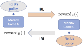
We leverage single-agent IRL for multi-agent Markov Games through an alternating learning framework. Given observations of two teams A and B, we first treat team B as part of A's environment, then learn a reward function for team A in a single-agent Markov decision process (MDP). The procedure is repeated with the role of teams A and B reversed. We give a mathematical justification for this procedure in the sense that the single-agent MDP value function for one team agrees with its Markov Game value function. We apply alternation to generic Home and Away teams.
As in previous RL work, the Q-function can be used to value actions and rank players. We apply IRL-DK to the 2018-19 play-by-play data in the NHL. The resulting distribution of top players is mixed among offensive and defensive players rather than concentrated among offensive players. Empirical comparison among 7 player evaluation metrics shows the high correlations with standard success measures and temporal consistency of our method.
Contributions. Our main contributions may be summarized as follows.
- A novel application of IRL to learning reward for teams in professional sports. Our method is general and can be applied to multi-agent dynamics in other domains.
- A transfer learning method for combining sparse explicit rewards with learned dense implicit rewards.
- An alternating learning procedure for leveraging singleagent IRL: For each agent in turn, the other agents are treated as part of the environment to define a singleagent MDP. We justify this procedure theoretically.
2 RelatedWork
We discuss previous work most related to our approach.
Player Evaluation. Most approaches use the total value of a player's actions to rank players [Albert et al., 2017]. This reduces player evaluation to action evaluation. One approach to defining expected impact for all actions is to train a classifier to predict whether an action will be followed by a goal within a fixed look-ahead horizon. A recent example is the VAEP method [Decroos et al., 2019] (see Sec. 8). State-ofthe-art methods use Q-function learning to assess the probability of scoring the next goal after a player's action. Examples include Scoring Impact [Routley and Schulte, 2015] and the GIM metric [Liu and Schulte, 2018] (see Sec. 8).
Multi-agent IRL is much less researched than single-agent IRL. A novel aspect of our work is combining learned rewards with explicitly observed rewards specified by domain knowledge. The most closely related work applies singleagent IRL to learn an individual reward function for World of Warcraft players [Wang et al., 2019]. They aim to model individual motivations, not to value actions and rank players.
Our work uses IRL for describing agent behaviour, whereas most other IRL work has the control objective of building optimal agents. Previous work assumes that expert agents are following a Nash equilibrium distribution, which defines optimality in Markov Games [Yu et al., 2019; Wang and Klabjan, 2018]. Our optimality assumption is related but fundamentally different: Let ˆπA,ˆπB be two policies for agents A and B estimated directly from the data that represent the agents' observed behaviour (cf. Sec. 4). Let ˆ rA and ˆ rB be two internal reward functions inferred from the data, where πrA A and πrB B are the inferred policies that optimize the agents' respective inferred reward functions. Our assumption is that agents optimize against the observed policies of other agents (i.e., ˆπA and ˆπB form an approximate Nash equilibrium). Previous control work computes policies such that agents optimize against the inferred optimal policies of other agents (i.e., π ˆ rA A and π ˆ rB B form an approximate Nash equilibrium). For describing a real-world domain like sports, our assumption is more realistic because i) teams have direct access only to the observed behavior of other teams, not to others' internal strategies (π ˆ r ), and ii) when an opponent's observed behavior ˆπ falls shorts of their optimal strategy π ˆ r , successful teams take advantage of it.
IRL and Knowledge Transfer. Mendez et al. (2018) consider reward knowledge transfer among multiple tasks in an on-line setting. We consider knowledge transfer between two reward functions for the same task. Wulfmeier et al. (2016) incorporate a known reward function using pretraining. We also initialize our model with pre-trained parameters consistent with domain knowledge, but further use a Gaussian kernel regularization during training.
3 Markov Game Model for Ice Hockey
We review the Markov Game formalism and show how it can be applied to ice hockey.
3.1 Markov Games and Decision Processes
Markov Games [Littman, 1994] extend MDPs to game theory [Von Neumann and Morgenstern, 1947]. Formally, a Markov Game [Littman, 1994] can be represented as a tuple G = 〈S,A, r, γ, T〉, where S is a finite set of states, A = (A1, . . . ,Ak) is a collection of finite action sets, one for each agent 1, . . . , k. For each agent, there is a real-valued reward function ri : S×Ai → R, and a shared discount factor 0 < γ < 1. The transition function T : S×A → PD(S) represents the environmental dynamics. (The notation PD(X) denotes the set of probability distributions over a finite set X.) An MDP is a single-agent Markov Game with k = 1.
A policy for agent i is a mapping πi : S → PD(Ai). We assume the on-policy setting with a fixed policy vector π1, . . . , πk. Note that since an agent's action probability is a function of the current game state, the agents' actions are independent of each other given the current game state. Focusing on a single agent i, we adopt game theory notation where
-i refers to the vector of the k-1 other agents. For instance, a policy vector can be decomposed as π = (πi, π-i). Given a policy vector, a Markov Game defines a game value function for each agent i and state, which we denote by Gπi,π-i i (s). The game value represents the expected cumulative reward for agent i if the game starts in the state s, and satisfies the Bellman equation:
where a-i = (a1, . . . , ai-1, ai+1, . . . , ak) is a vector of actions by the agents other than i, and π-i(a-i|s) is the probability of these independent actions given the policies of the agents other than i. This Bellman equation has a unique solution [Sutton and Barto, 1998].
3.2 Ice HockeyMarkov Game
Ice hockey is one of the four major sports played in North America. Each team tends a goal. Players skate on ice controlling a puck with a stick. A team scores a goal when it moves the puck into the the opposing team's goal. The match winner is the team with the most goals. A complete list of rules is available on-line (www.nhl.com).
We utilize a proprietary play-by-play dataset constructed by SPORTLOGiQ company. This dataset captures information of the NHL games from October 2018 to April 2019, which contains 4,534,017 events, covering 31 teams, 979 players and 1,202 games. The data consists of game events around the puck, including the location and timestamp of a certain event, the identity of the player in possession and the action taken by this player, and other game context features (score difference, manpower, period, etc.). The X and Y coordinates are adjusted to the range [-100, 100] and [-42.5, 42.5] in feet, where the origin is center ice, the x-axis is along the length of the rink, and the y-axis is along the width.
As in previous work, [Routley and Schulte, 2015; Schulte et al., 2017] our Markov Game model for ice hockey uses a factored state space where a state is a list of values for features that represent the match context. The features include game context, team identity (H/A) and location (L). A game context comprises Goal Difference (GD), ManPower (MP), and Period (P). GD is calculated as the number of home goals minus the number of away goals, ranging from -8 to 8. MP specifies shorthanded, even strength, and powerplay. P represents the current period, ranging from 1 to 3. (We do not consider overtime play.) We divide the hockey rink into 6 regions indexed by L based on the two blue lines to divide the X axis. We add an absorbing goal state for each team, with no transition out of it. The dataset records 27 different action types, and home and away teams share the same action space. We treat home team H and away team A as two agents in the game. At each timestamp, only one agent performs an action, and the agent not controlling the puck chooses no operation.
As in previous work [Routley and Schulte, 2015], each ice hockey game is modeled as a semi-episodic task [Sutton and Barto, 1998], where games switch from episode to episode. Each episode starts either at the beginning of the game or right after a goal, and ends up with a goal or the end of the game. The transition function is calculated using the observed frequency T(s, a, s′ ) = p(s′ |s, a) = O(s, a, s′ )/O(s, a), where O(·) counts the occurrence number in our dataset.
4 Alternating Learning for Multi-Agent IRL
Figure 1 illustrates the system flow of our alternating IRL for two agents A and B. First, estimate a policy ˆπB for agent B. Given the policy ˆπB, agent B can be treated as part of the environment for agent A. This reduces learning a reward function for agent A to a single-agent problem. Second, we repeat this procedure, with the roles of A and B reversed. Since the estimated policies for each team do not change, the loop is not repeated more than once.
The following definitions formalize this design and support a theoretical justification: We show that given a fixed policy vector π-i, from agent i's perspective, a Markov Game G = 〈S, A, r, γ, T 〉 is equivalent to a single-agent MDP. We define the marginal MDP as M(π-i) := 〈S,Ai, r′ , γ, T ′ 〉, where
- r′ (s, ai) = ∑a-i ri(s, ai, a-i) · π-i(a-i|s)
- T ′ (s′ |ai, s) = ∑a-i T (s′ |ai, a-i, s) · π-i(a-i|s).
Proposition 1. Given a Markov Game G and policy vector π-i for the agents other than i, the values of any policy πi for Algorithm 1 Alternating IRL for two agents Markov Game A and B.
Input: Partial Markov Game G = 〈S, AA, AB, γ, T 〉
Data: State-Action Event Data D
Output: Learned reward functions ˆ rA and ˆ rB
Calls: Single-Agent IRL procedure φ that learns reward ˆ r = φ(M, D) given MDP M \ r, D
- 1: estimate maximum-likelihood policy ˆπB from data D
- 2: T ′ (s′ |aA, s) = ∑aB T(s′ |aA, aB, s) · ˆπB(aB|s)
- 3: partial MDPM \ r := 〈S,AA, γ, T ′ 〉
- 4: ˆ rA := φ(M,D).
/*end learning reward for agent A*/
- 5: estimate maximum-likelihood policy ˆπA from data D
- 6: T ′ (s′ |aB, s) = ∑aA T(s′ |aA, aB, s) · ˆπA(aA|s)
- 7: partial MDPM \ r := 〈S,AB, γ, T ′ 〉
- 8: ˆ
- rB := φ(M,D). /*end learning reward for agent B*/
- 9: return ˆ rA, ˆ rB
agent i is the same in G and the marginal MDP M(π-i):
The proof is in the Appendix. Algorithm 1 gives pseudocode for leveraging single-agent IRL based on Proposition 1. In our sports application, A represents a generic Home team, and B a generic Away team. We show in Section 5 the design of a single-agent procedure φ to incorporate sparse observed rewards (which in our sports application represent goals).
5 IRL with Domain Knowledge
We use alternating learning procedure to leverage any singleagent IRL procedure φ for a multi-agent Markov Game. For our experiments, we choose maximum entropy (MaxEnt) IRL because it provides an interpretable linear model for a reward function and scales to our large dataset. We first review the basic method and then present a new contribution: showing how MaxEnt IRL can be extended to incorporate domain knowledge in the form of explicitly given reward labels.
5.1 MaximumEntropy IRL
In MaxEnt IRL [Ziebart et al., 2008], each state s is assigned a feature vector fs ∈ Rk , and the reward function is parameterized as a linear function of a state with reward weights θ ∈ Rk as rθ(s) = θTfs. The state reward can be interpreted as the expected value over actions of the MDP reward r(s, a). The reward value for a trajectory ζ is simply the cumulative reward of visited states,
where fζ = ∑sj∈ζ fsj is called the feature count of the trajectory. The observed agents' feature counts are calculated as ˜ f = 1m ∑ζ fζ , where m is the number of trajectories.
Assuming that agents follow a maximum entropy [Jaynes, 1957] policy, the probability of a demonstrated trajectory ζ increases exponentially with higher rewards. Eq. 4 in [Ziebart et al., 2008] shows that under mild assumptions, the exponential trajectory probability can be approximated by the expression
where Z(θ, T ) is the partition function and T is the state transition distribution. Fixing T, the optimal ˆ θ maximizes the log-likelihood L(θ) of the demonstrations
The maximum is obtained using gradient ascent; the gradient of L(θ) is the difference between observed and expected feature counts, which can be expressed in terms of state visitation frequencies Ds. The frequency of visiting a state given a policy can be computed with an iterative algorithm
5.2 MaxEnt IRL with Domain Knowledge
Directly using an IRL algorithm to recover the reward function from game dynamics models what situations professional players want to be in, that is, their internal reward function rθ. But the MaxEnt approach fails to learn the importance of goals in a game, mainly because goals are such rare events in ice hockey. Previous RL methods define the reward function explicitly in terms of goals. The rule reward function rK (for knowledge) assigns reward 1 for scoring a goal (i.e., getting the puck into the net) and 0 for other actions. Our knowledge transfer approach combines the MaxEnt likelihood function with the goal reward function through regularization:
where rθ = θTψ, rK = θTK ψ, ψ = [fs1 , ..., fsn ] ∈ Rk×n is the state feature matrix, λ is a trade-off parameter, and k is a kernel function that bridges the disparity between learned and knowledge reward functions. In this paper we use a Gaussian kernel k(xi, xj) = exp{-||xi - xj||2 /2}. Following [Wulfmeier et al., 2016], we pre-train a parameter vector θK to match our domain knowledge rK and initialize θ with θK. The gradient for θ is given by
This completes the description of our learning method. We next derive the regularizer (6) from a previous knowledge transfer framework.
Maximum Mean Discrepancy (MMD) [Gretton et al., 2012] is an established framework for transferring knowledge between two distributions over random variables. Let X and Y be two random variables. Formally, MMD defines the following difference measure
where Hk endowed by a kernel function k(x, x′ ) is a Hilbert space of functions f(x) → R with inner product, known as a reproducing kernel Hilbert space (RKHS) [Gretton et al., 2012]. Given observations x of X and y of Y , an unbiased estimation of squared MMD is given by:
Since ˆ θ is a function of a sample, it denotes a random variable. As a result, rˆ θ also defines a random variable, which we denote as Rˆ θ with observation rˆ θ . We also associate with rK a constant random variable RK with observation rK.
As kernel function k is a Gaussian kernel in most knowledge transfer frameworks [Long et al., 2017], the optimal ˆ θ is derived byˆ
where we have used the fact that the first two terms in Equation (9) are constant for a Gaussian kernel. Setting λ = 2α yields Equation (6).
6 Evaluating the Learned Reward and Policy
We examine two IRL methods for sports data that apply the alternating algorithm 1 with two different single-agent IRL procedures φ. IRL-DK is our full method, with regularized MaxEnt objective (6). IRL maximizes the MaxEnt objective (4) without regularization. Hyperparameters were set as follows. λ = 1 for IRL-DK, λ = 0 for IRL. Discount factor γ = 0.9 for all methods. The learning rate for gradient ascent was 0.001, set for optimum convergence. 1
We report different properties of the IRL-DK learned reward function from the ice hockey data.
Reward Density. Since our goal is to complement the sparse observed rewards with a dense reward signal that covers many situations, we would want the variance of learned rewards to be substantially higher than that of goal rewards. Table 1 verifies that this is the case: the standard deviation (STD) of learned rewards is an order of magnitude higher, and the STD of the Q-function derived from the learned rewards is two orders of magnitude higher than that of the Q-function derived from goal rewards. The computation of the Q-values for IRL-DK is discussed in Section 7.1. For the goal reward function, we used the Q-values provided by [Liu and Schulte, 2018], the state-of-the-art RL method for the goal reward.
Policy Evaluation. To evaluate how well the reward function recovered by our model rationalizes players' behavior, we solve the MDP for the learned reward functions to obtain two optimal policies π ˆ θH and π ˆ θA for the home and away teams respectively. Then we compare the demonstrated trajectories with the probabilistic distribution over trajectories generated by the policies, using two common metrics: negative log-likelihood (NLL) and modified Hausdorff Distance (MHD) [Wulfmeier et al., 2016].
1 Code available at https://github.com/miyunluo/IRL-icehockey.
| Items | Mean | STD |
|---|---|---|
| Rule reward function (goals) | 0.0000 | 0.0383 |
| IRL-DK learned reward function | 0.7964 | 0.1281 |
| Q-values from goals (GIM) | 0.4222 | 0.0963 |
| Q-values from IRL-DK | 5.1863 | 1.2207 |
NLL calculates how likely the demonstrations are under policy π, and MHD is a spatial measure of the distance between demonstrated and generated trajectories. Table 2 shows the average results for both home/away teams. The policies optimal for the IRL reward with domain knowledge outperform their counterparts on both metrics.
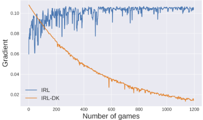
Learning Performance. Figure 2 shows the gradient changes during training for IRL and IRL-DK respectively. IRL is very unstable with oscillating gradients and fails to completely converge. Combining IRL with domain knowledge leads to a smoother training and faster convergence.
| Methods | NLL | HMD |
|---|---|---|
| Rule reward function (goals) | 185.0 | 13.37 |
| IRL learned reward function | 53.9 | 9.71 |
| IRL-DK learned reward function | 49.5 | 7.77 |
7 Player Ranking
We assess the learned reward function in a downstream application, player ranking. We first define the action impact values and then give examples of player ranking.
7.1 Action Impact Values
Action impact, which quantifies the difference made by an action, has been used for player evaluation [Routley and Schulte, 2015; Schulte et al., 2017; Liu and Schulte, 2018]. We adopt action impact values as a function of game context (Markov state) [Routley and Schulte, 2015]. For the home teamH, the impact is defined by
where H is the team executing the action a, and the policy π ˆ θH is obtained by solving the single-agent MDP for the home team given the learned reward (cf. Section 6). Impact for the away team is defined similarly. The action impact function measures how much an action improves over the average action.
7.2 Player Rankings
Following [Liu and Schulte, 2018], the ranking score for a player is the sum of this player's total action impact values
where D denotes our dataset, i is the playerId, niD (s, a) is the occurrence number that player i performed action a at state s observed fromD, and teami is the team of player i. The total impact is not normalized for time-on-ice (TOI), because TOI correlates with player strength. Dividing the ranking score by TOI therefore reduces the score differences among players. Note that impact values can be both positive and negative, so the total impact reflects the net value of a player's actions, rather than the total number of the actions.
Different from [Routley and Schulte, 2015; Liu and Schulte, 2018] where all the players are evaluated together, we evaluate offensive players (Center, Left Wing, Right Wing) and defensive players (Defenceman, Goalie) separately with the following considerations. First, previous RL methods with sparse reward rank offensive players higher than defensive players in most cases. Second, these two types of players play different roles in a team under diverse strategies leading to distinct behavior.
Tables 3 and 4 list the top-10 highest impacts offensive and defensive players by our algorithm. All these players are fantasy NHL stars according to recent NHL 2019-20 top players news. Our ranking can be used to identify promising players. For instance, Miro Heiskane just began his career in 2017 and drew salaries below other top ranking players but is nominated as a top-50 defenceman by NHL [Reese, 2019]. Our ranking does not have apparent bias towards offensive players compared with two recent RL methods, Score Impact (SI) [Routley and Schulte, 2015] and Goal Impact Metric (GIM) [Liu and Schulte, 2018]. For instance, comparing the top-50 players, for the SI metric they are all offensive players, for GIM all but one are offensive player, whereas our method contains 32 defencemen.
| Name | Assists | Goals | Points | Team | Salary |
|---|---|---|---|---|---|
| Anze Kopitar | 38 | 22 | 60 | LA | 11,000,000 |
| Aleksander Barkov | 61 | 35 | 96 | FLA | 6,900,000 |
| Dylan Larkin | 41 | 32 | 73 | DET | 7,000,000 |
| Nathan Mackinnon | 58 | 41 | 99 | COL | 6,750,000 |
| Leon Draisaitl | 55 | 50 | 105 | EDM | 9,000,000 |
| Mark Scheifele | 46 | 38 | 84 | WPG | 6,750,000 |
| Jonthan Toews | 46 | 35 | 81 | CHI | 9,800,000 |
| Connor McDavid | 75 | 41 | 116 | EDM | 14,000,000 |
| Jack Eichel | 54 | 28 | 82 | BUF | 10,000,000 |
| Ryan O'Reilly | 53 | 30 | 83 | CAR | 6,000,000 |
| Name | Assists | Goals | Points | Team | Salary |
|---|---|---|---|---|---|
| Drew Doughty | 37 | 8 | 45 | LA | 12,000,000 |
| Brent Burns | 67 | 16 | 83 | SJ | 10,000,000 |
| Roman Josi | 41 | 15 | 56 | NSH | 4,000,000 |
| John Carlson | 57 | 13 | 70 | WSH | 12,000,000 |
| Morgan Rielly | 52 | 20 | 72 | TOR | 5,000,000 |
| Ryan Suter | 40 | 7 | 47 | MIN | 9,000,000 |
| Mark Giordano | 57 | 17 | 74 | CGY | 6,750,000 |
| Duncan Keith | 34 | 6 | 40 | CHI | 3,500,000 |
| Erik Gustafsson | 43 | 17 | 60 | CHI | 1,800,000 |
| Miro Heiskane | 21 | 12 | 33 | DAL | 925,000 |
8 Player Ranking Empirical Evaluation
Similar to clustering problems, there is no ground truth for player evaluation. To assess player evaluation metrics, we follow previous work [Routley and Schulte, 2015; Schulte et al., 2017; Liu and Schulte, 2018] and compute their correlation with commonly used statistic measurements like Assists, Goals, Points, as these statistics are generally regarded as important measures of a player's ability to impact a game.
We compare our method with the following player evaluation metrics. Metrics derived from a Markov model include SI and GIM. These metrics use only the observed goal reward, no inferred rewards. Scoring Impact (SI) is most related to our method, also based on a discrete Markov Game model [Routley and Schulte, 2015; Schulte et al., 2017]. Goal Impact Metric (GIM) uses a deep Q-network to predict Q-values and defines the difference between two consecutive Q-values as action impact [Liu and Schulte, 2018].
We also compare a number of player metrics not based on a Markov model. Plus-minus (+/-) is a commonly used basic metric to measure the influence of player presence on goal scoring [Macdonald, 2011]. Win-Above-Replacement (WAR) estimates the difference of team's wining chance if a target player is replaced by an average player [Gerstenberg et al., 2014]. Expected Goal (EG) weights each shot by its chance of leading to a goal [Macdonald, 2012]. Valuing Actions by Estimating Probabilities (VAEP) defines the impact of an action as its offensive score plus defensive score [Decroos et al., 2019]. These two scores are defined as the differences between two consecutive scoring and conceding probabilities.
8.1 Season Totals: Correlations with Standard Success Measures
The following experiment computes the correlations with success measures over the entire 2018-19 season. The NHL official website provides 14 standard success measures (www.nhl.com/stats/player), including Assists, Goals, Points, Game Play (GP), Game Wining Goal (GWG), Shorthanded Goal (SHG), Power-play Goal (PPG), Shots (S), Short-handed Point (SHP), Power-play Point (PPP), Face-off Win Percentage (FOW), Points per game (P/GP), Shifts per game (SFT/GP), and Penalty Minute (PIM). The results for offensive and defensive players are shown in Tables 5 and 6.
| Methods | Assists | GP | Goals | GWG | SHG | PPG | S |
|---|---|---|---|---|---|---|---|
| +/- | 0.269 | 0.086 | 0.282 | 0.278 | 0.118 | 0.124 | 0.156 |
| VAEP | 0.215 | 0.185 | 0.215 | 0.089 | -0.074 | 0.160 | 0.239 |
| WAR | 0.591 | 0.322 | 0.742 | 0.571 | 0.179 | 0.610 | 0.576 |
| EG | 0.656 | 0.629 | 0.633 | 0.489 | 0.099 | 0.391 | 0.737 |
| SI | 0.717 | 0.633 | 0.975 | 0.665 | 0.249 | 0.770 | 0.860 |
| GIM | 0.757 | 0.772 | 0.781 | 0.518 | 0.147 | 0.477 | 0.795 |
| IRL | 0.855 | 0.872 | 0.812 | 0.587 | 0.123 | 0.513 | 0.901 |
| IRL-DK | 0.882 | 0.887 | 0.824 | 0.607 | 0.125 | 0.537 | 0.907 |
| Methods | Points | SHP | PPP | FOW | P/GP | SFT/GP | PIM |
| +/- | 0.285 | 0.179 | 0.157 | 0.012 | 0.306 | 0.109 | 0.100 |
| VAEP | 0.235 | -0.076 | 0.185 | 0.021 | 0.204 | 0.129 | 0.172 |
| WAR | 0.692 | 0.147 | 0.605 | 0.040 | 0.699 | 0.396 | 0.145 |
| EG | 0.694 | 0.183 | 0.508 | 0.254 | 0.644 | 0.713 | 0.355 |
| SI | 0.869 | 0.204 | 0.708 | 0.135 | 0.728 | 0.639 | 0.361 |
| GIM | 0.818 | 0.151 | 0.561 | 0.289 | 0.705 | 0.751 | 0.372 |
| IRL | 0.891 | 0.207 | 0.696 | 0.294 | 0.741 | 0.818 | 0.437 |
| IRL-DK | 0.908 | 0.213 | 0.734 | 0.298 | 0.769 | 0.820 | 0.446 |
| Methods | Assists | GP | Goals | GWG | SHG | PPG | S |
|---|---|---|---|---|---|---|---|
| +/- | 0.173 | 0.132 | 0.144 | 0.177 | 0.235 | -0.116 | 0.113 |
| VAEP | 0.054 | -0.045 | 0.005 | 0.010 | 0.384 | 0.071 | -0.016 |
| WAR | 0.204 | 0.028 | 0.365 | 0.275 | 0.097 | 0.246 | 0.186 |
| EG | 0.589 | 0.688 | 0.507 | 0.321 | 0.327 | 0.306 | 0.679 |
| SI | 0.607 | 0.488 | 0.934 | 0.449 | 0.491 | 0.457 | 0.709 |
| GIM | 0.702 | 0.862 | 0.596 | 0.263 | 0.130 | 0.170 | 0.764 |
| IRL | 0.809 | 0.941 | 0.686 | 0.415 | 0.268 | 0.347 | 0.908 |
| IRL-DK | 0.852 | 0.959 | 0.701 | 0.439 | 0.289 | 0.360 | 0.920 |
| Methods | Points | SHP | PPP | FOW | P/GP | SFT/GP | PIM |
| +/- | 0.175 | 0.107 | -0.05 | 0.095 | 0.169 | 0.067 | 0.072 |
| VAEP | 0.042 | 0.065 | -0.003 | 0.101 | 0.064 | -0.036 | -0.031 |
| WAR | 0.252 | 0.128 | 0.266 | 0.174 | 0.279 | 0.006 | -0.089 |
| EG | 0.611 | 0.278 | 0.399 | 0.118 | 0.503 | 0.694 | 0.360 |
| SI | 0.720 | 0.174 | 0.488 | 0.103 | 0.521 | 0.499 | 0.272 |
| GIM | 0.730 | 0.085 | 0.358 | 0.140 | 0.471 | 0.706 | 0.438 |
| IRL | 0.841 | 0.281 | 0.549 | 0.182 | 0.557 | 0.776 | 0.549 |
| IRL-DK | 0.865 | 0.307 | 0.571 | 0.185 | 0.574 | 0.778 | 0.570 |
Our method achieves the highest correlation in 10 out of 14 success measures except for goal and three goal related items (GWG, SHG, and PPG). For these measures, only SI shows a higher correlation, because it is dominated by goal action. For GWG, our results are comparable to SI for both offensive and defensive player measures. For SHG and PPG, it achieves the second best results or comparable to the second best. The traditional plus-minus correlates poorly with all success measures. VAEP only achieves little correlation with success measures because their model is a classifier built on data with few positive labels and tends to assign similar impact value to all actions. EG is only the fourth best metric, because it only takes shots into account. IRL-DK achieves higher correlations than GIM, the most recent method, for every success measure except for SHG. The difference is especially pronounced for defencemen and non-goal related measures (e.g. points), due to GIM's goal bias. Compared to the no-knowledge IRL baseline, the correlations of IRL-DK are consistently higher but not by much. This is evidence that providing a denser reward signal with either inverse RL method improves player rankings.
8.2 Round-by-Round Correlations: Predicting Future Performance from Past Performance
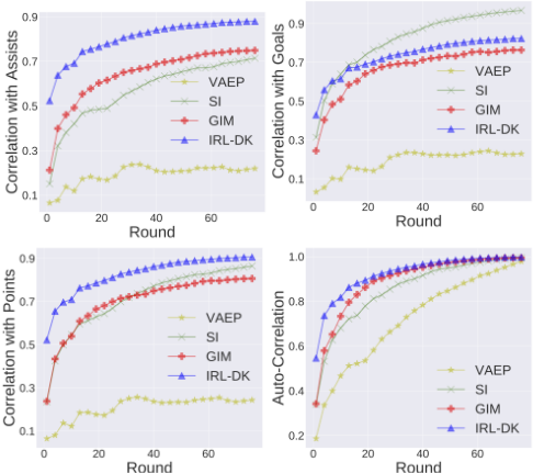
A sport season normally consists of several rounds. A team or player will finish n competitions at the end of round n. We compute the correlation between player values at the end of round n and three main success measures, Assists, Goals, and Points, over the whole sport season. This experiment assesses the predictive power of different metrics, which allow us to infer the future performance of players. We also compute the auto-correlation for different metrics between players' round values and final season values. Auto-correlation evaluates the temporal consistency of a metric [Pettigrew, 2015]. Since most players' strengths are stable throughout a season, a good player metric should show temporal consistency.
We focus on the four machine learning methods VAEP, SI, GIM, and IRL-DK. Figure 3 shows round-by-round correlation with Assists, Goals, Points, and the auto-correlation between round values and season total for offensive players. (Results for defensive players are similar, but not shown due to the page limit.) IRL-DK is the most stable model measured by auto-correlation, and is the best at predicting success measures, even at the very beginning of the season.
9 Conclusion
We investigated multi-agent inverse reinforcement learning for professional ice hockey game analytics, a novel application area for AI. Our aim was to recover reward for complex game dynamics, which addresses the sparse reward issue for RL models. We introduced a transfer learning based regularization approach to incorporate domain knowledge in IRL. Based on the recovered reward function and calculated Q-values, we computed a context-aware player performance metric that provides a comprehensive evaluation for both offensive and defensive players in NHL by taking all their actions into account. In experiments our method shows no obvious bias for any player position, achieves highest correlation with most standard success measures among competing methods, and is most temporally consistent. While we have focused on ice hockey for concreteness, the IRL with domain knowledge method can be easily applied to a Markov Game model for any similar team sport. Another important direction for future work is to learn reward functions at different levels, for instance, for individual teams and players.
Acknowledgments
This work was supported by a Strategic Project Grant from the Canadian Natural Sciences and Engineering Research Council (NSERC).
A Proof of Proposition 1
We show that the Bellman equation for the marginal MDP is the same as for the Markov Game. Since each Bellman equation has a unique value function as a solution, this implies that the value functions are the same.
The value function of a marginal MDP (Sec. 4) is
This equation agrees with the Markov Game value function.
B VAEP Implementation
VAEP probabilities are estimated by building a probabilistic binary classifier for predicting whether a given possession will end in a goal. The original VAEP work [Decroos et al., 2018], utilized both a neural network and a tree classifier, and reported very similar performance for both. Our dataset contains 4.5M records, whereas the VAEP dataset posted online contains only 2.7M. In most recent version [Decroos et al., 2019], a gradient-boosted tree was applied to a dataset of over 11K games, but we were not able to scale the on-line code to our dataset (https://github.com/ML-KULeuven/socce raction). Instead, we utilized a neural network with an LSTM layer followed by two fully connected layers (100 and 50 ReLU nodes), and a sigmoid output layer. The trace length of LSTM is 10, corresponding to the VAEP default look-ahead of k = 10. We trained for 10 epochs on the whole dataset.
@inproceedings{ijcai2020p464,
  title     = {Inverse Reinforcement Learning for Team Sports: Valuing Actions and Players},
  author    = {Luo, Yudong and Schulte, Oliver and Poupart, Pascal},
  booktitle = {Proceedings of the Twenty-Ninth International Joint Conference on
               Artificial Intelligence, {IJCAI-20}},
  publisher = {International Joint Conferences on Artificial Intelligence Organization},
  editor    = {Christian Bessiere},
  pages     = {3356--3363},
  year      = {2020},
  month     = {7},
  note      = {Main track},
  doi       = {10.24963/ijcai.2020/464},
  url       = {https://doi.org/10.24963/ijcai.2020/464},
}
TY - CPAPER TI - Inverse Reinforcement Learning for Team Sports: Valuing Actions and Players AU - Luo, Yudong AU - Schulte, Oliver AU - Poupart, Pascal T2 - Proceedings of the Twenty-Ninth International Joint Conference on Artificial Intelligence, IJCAI-20 PB - International Joint Conferences on Artificial Intelligence Organization PY - 2020 SP - 3356 EP - 3363 DO - 10.24963/ijcai.2020/464 UR - https://doi.org/10.24963/ijcai.2020/464 ER -Copied
Machine-readable versions of this paper, for tools and AI agents:





