
Iterative-Deepening Conflict-Based Search
Proceedings of the Twenty-Ninth International Joint Conference on Artificial Intelligence. Main track. Pages 4084-4090.
https://doi.org/10.24963/ijcai.2020/565
Keywords
- Planning and Scheduling: Planning and Scheduling
- Heuristic Search and Game Playing: Heuristic Search
- Agent-based and Multi-agent Systems: Multi-agent Planning
Abstract
Conflict-Based Search (CBS) is a leading algorithm for optimal Multi-Agent Path Finding (MAPF). CBS variants typically compute MAPF solutions using some form of A* search. However, they often do so under strict time limits so as to avoid exhausting the available memory. In this paper, we present IDCBS, an iterative-deepening variant of CBS which can be executed without exhausting the memory and without strict time limits. IDCBS can be substantially faster than CBS due to incremental methods that it uses when processing CBS nodes.
- [Barer et al., 2014] Max Barer, Guni Sharon, Roni Stern, and Ariel Felner. Suboptimal variants of the conflict-based search algorithm for the multi-agent pathfinding problem. Proceedings of the Annual Symposium on Combinatorial Search (SoCS-2014), pages 19-27, 2014.
- [Boyarski et al., 2015a] Eli Boyarski, Ariel Feiner, Guni Sharon, and Roni Stern. Don't split, try to work it out: By- passing conflicts in multi-agent pathfinding. In Proceed- ings of the International Conference on Automated Plan- ning and Scheduling (ICAPS-2015), pages 47-51, 2015.
- [Boyarski et al., 2015b] Eli Boyarski, Ariel Felner, Roni Stern, Guni Sharon, David Tolpin, Oded Betzalel, and Eyal S. Shimony. ICBS: Improved conflict-based search algorithm for multi-agent pathfinding. In Proceedings of the International Joint Conference on Artificial Intel- ligence (IJCAI-2019), pages 740-746, 2015. IJCAI
- [Felner et al., 2017] Ariel Felner, Roni Stern, Solomon Eyal Shimony, Eli Boyarski, Meir Goldenberg, Guni Sharon, Nathan Sturtevant, Glenn Wagner, and Pavel Surynek. Search-based optimal solvers for the multi-agent pathfind- ing problem: Summary and challenges. In Proceedings of the Annual Symposium on Combinatorial Search (SoCS- 2017), pages 29-37, 2017.
- [Felner et al., 2018] Ariel Felner, Jiaoyang Li, Eli Boyarski, Hang Ma, Liron Cohen, T. K. Satish Kumar, and Sven Koenig. Adding heuristics to conflict-based search for multi-agent path finding. In Proceedings of the Interna- tional Conference on Automated Planning and Scheduling (ICAPS-2018), pages 83-87, 2018.
- [Gange et al., 2019] Graeme Gange, Daniel Harabor, and Peter J. Stuckey. Lazy CBS: Implicit conflict-based search using lazy clause generation. In Nir Lipovetzky, Eva On- aindia, and David Smith, editors, Proceedings of the Inter- national Conference on Automated Planning and Schedul- ing (ICAPS-2019), pages 155-162. AAAI Press, 2019.
- [Koenig et al., 2004] Sven Koenig, Max Likhachev, and David Furcy. Lifelong planning A*. Artificial Intelligence, 155(1-2):93-146, 2004.
- [Korf, 1985] Richard Korf. Depth-first iterative-deepening: An optimal admissible tree search. Artificial Intelligence, 27(1):97-109, 1985.
- [Kou et al., 2020] Ngai Meng Kou, Cheng Peng, Hang Ma, T. K. Satish Kumar, and Sven Koenig. Idle time optimiza- tion for target assignment and path finding in sortation cen- ters. In Proceedings of the AAAI Conference on Artificial Intelligence (AAAI-2020), 2020.
- [Li et al., 2019a] Jiaoyang Li, Ariel Felner, Eli Boyarski, Hang Ma, and Sven Koenig. Improved heuristics for multi- agent path finding with conflict-based search. In Proceed- ings of the International Joint Conference on Artificial In- telligence (IJCAI-2019), pages 442-449, 2019.
- [Li et al., 2019b] Jiaoyang Li, Daniel Harabor, Peter J Stuckey, Hang Ma, and Sven Koenig. Disjoint splitting for multi-agent path finding with conflict-based search. In Proceedings of the International Conference on Au- tomated Planning and Scheduling (ICAPS-2019), pages 279-283, 2019.
- [Li et al., 2019c] Jiaoyang Li, Daniel Harabor, Peter J. Stuckey, Hang Ma, and Sven Koenig. Symmetry-breaking constraints for grid-based multi-agent path finding. In Pro- ceedings of the AAAI Conference on Artificial Intelligence (AAAI-2019), pages 6087-6095, 2019.
- [Ma et al., 2016] Hang Ma, Sven Koenig, Nora Ayanian, Liron Cohen, Wolfgang Hönig, T. K. Satish Kumar, Tansel Uras, Hong Xu, C. Tovey, and G. Sharon. Overview: Gen- eralizations of multi-agent path finding to real-world sce- narios. In IJCAI-16 Workshop on Multi-Agent Path Find- ing, 2016.
- [Ma et al., 2019] Hang Ma, Daniel Harabor, Peter J. Stuckey, Jiaoyang Li, and Sven Koenig. Searching with consistent prioritization for multi-agent path finding. In Proceedings of the AAAI Conference on Artificial Intelligence (AAAI- 2019), pages 7643-7650. AAAI Press, 2019.
- [Okoso et al., 2019] Ayano Okoso, Keisuke Otaki, and Tomoki Nishi. Multi-agent path finding with priority for cooperative automated valet parking. In Proceedings of the IEEE Intelligent Transportation Systems Conference (ITSC-2019), pages 2135-2140, 2019.
- [Ruml, 2010] Wheeler Ruml. The logic of benchmarking: A case against state-of-the-art performance. In Proceedings of the 3rd Annual Symposium on Combinatorial Search (SoCS-2010), pages 142-143, 2010.
- [Sharon et al., 2013] Guni Sharon, Roni Stern, Meir Gold- enberg, and Ariel Felner. The increasing cost tree search for optimal multi-agent pathfinding. Artificial Intelligence, 195(Supplement C):470 -495, 2013.
- [Sharon et al., 2015] Guni Sharon, Roni Stern, Ariel Fel- ner, and Nathan R Sturtevant. Conflict-based search for optimal multi-agent pathfinding. Artificial Intelligence, 219:40-66, 2015.
- [Silver, 2006] David Silver. Cooperative pathfinding. In Steve Rabin, editor, AI Game Programming Wisdom 3, pages 99-111. 2006.
- [Standley, 2010] Trevor Standley. Finding optimal solutions to cooperative pathfinding problems. In Proceedings of the AAAI Conference on Artificial Intelligence (AAAI-2010), pages 173-178, 2010.
- [Stern et al., 2019] Roni Stern, Nathan R. Sturtevant, Ariel Felner, Sven Koenig, Hang Ma, Thayne T. Walker, Jiaoyang Li, Dor Atzmon, Liron Cohen, T. K. Satish Kumar, Roman Barták, and Eli Boyarski. Multi-agent pathfinding: Definitions, variants, and benchmarks. In Proceedings of the Annual Symposium on Combinatorial Search (SoCS-2019), pages 151-159, 2019.
- [Surynek, 2018] Pavel Surynek. A summary of adaptation of techniques from search-based optimal multi-agent path finding solvers to compilation-based approach. CoRR, abs/1812.10851, 2018.
- [Wurman et al., 2008] Peter R. Wurman, Raffaello D'Andrea, and Mick Mountz. Coordinating hun- dreds of cooperative, autonomous vehicles in warehouses. AI Magazine, 29(1):9-19, 2008.
- [Yu and LaValle, 2016] Jingjin Yu and Steven M. LaValle. Optimal multirobot path planning on graphs: Complete al- gorithms and effective heuristics. IEEE Transactions on Robotics, 32(5):1163-1177, Oct 2016.
References were extracted automatically from the PDF and may contain errors.
Full text extracted automatically from the PDF; figures, tables and equations may differ. The PDF is the version of record.
1 Introduction
Multi-Agent Path Finding (MAPF) is a coordination problem which asks us to find a set of collision-free paths for a team of mobile agents, each from its start location to its designated goal location. MAPF is a well-known and well-studied topic with numerous real-world applications. For example, MAPF appears as a core challenge in automated warehouse logistics [Wurman et al., 2008], in automated parcel sortation [Kou et al., 2020], in automated valet parking [Okoso et al., 2019], in computer games [Silver, 2006] and in a variety of other contexts [Ma et al., 2016]. Many optimal MAPF solvers exist [Yu and LaValle, 2016; Surynek, 2018]. See also the survey by Felner et al. [2017].
Conflict-Based Search (CBS) [Sharon et al., 2015] is a popular two-level optimal MAPF solver. The low level finds optimal paths for the individual agents. If the paths include collisions, the high level, via a split action, imposes constraints on the agents to avoid these collisions. The search space of CBS is therefore a binary Conflict Tree (CT), which the algorithm explores in best-first order. CBS is complete, optimal and often highly performant; e.g., recent variants [Li et al., 2019a; 2019b; 2019c] can solve MAPF problem instances with > 100 agents. Unfortunately, all these algorithms suffer from the same significant drawback - as the search continues, they all need to store the entire search frontier, i.e., the entire open-list (OPEN), in memory. In CBS variants, the number of frontier nodes is exponential in the depth of the CT, which means that the available memory may be exhausted long before they have an opportunity to expand a goal node. For this reason, experiments with CBS are always executed with short time limits of 1 to 5 minutes. From a practical perspective, this means CBS will either find a solution quickly or fail and leave the practitioner without any recourse. There is no possibility to, e.g., allow the algorithm to run longer. 1
In this work, we first introduce Iterative-Deepening CBS (IDCBS), a new optimal MAPF algorithm which replaces the high-level A*-like search of CBS with a search like IDA*'s [Korf, 1985] which is a search algorithm for exponential domains that uses memory conservatively. IDCBS explores the CT using repeated depth-first iterations. Unlike A*, Depth-First Search (DFS) only moves from a parent node to its child and back and such nodes have many similarities in their content. This is a substantial change that requires some fundamental re-thinking of the CBS algorithm. Second, we identify 6 main components required to process a high-level CBS node and show how each one can be improved using incremental data structures that exploit similarities between parent nodes and their children. Third, we undertake an extensive empirical comparison which demonstrates practical benefits. IDCBS is able to optimally solve many more problem instances than CBS and we report substantial improvements in search times even for problem instances which can be solved by a currently leading CBS variant.
2 Definitions and Background
MAPF is defined by a graph G = (V,E) and a set of k agents {a1, . . . , ak}, where each agent ai has a start location starti ∈ V and a goal location goali ∈ V . We assume time is discretised into timesteps of unit size. At each timestep, every agent can either move to an adjacent vertex or wait at its current vertex. Moving and waiting both have a cost and, for simplicity and w.l.o.g., we assume this cost is 1.
A path for agent ai is a sequence of move/wait actions that takes the agent from starti to goali
are in collision (equivalently, in conflict) if they attempt to occupy the same vertex at the same timestep or if they attempt to traverse the same edge at the same timestep in different directions. To represent vertex conflicts we use the notation
1 Bounded-suboptimal variants of CBS [Barer et al., 2014] can mitigate this issue to a limited extent, but their memory consumption is still exponential in the depth of the CT.
1 Main(MAPF problem instance) 2 R←new CT node 3 R.constraints ← {} 4 R.solution ←{a shortest path for each agent} 5 R.cost ← SIC(R.solution) 6 R.conflicts ← Find Conflicts(R.solution) 7 Insert R into OPEN 8 while OPEN not empty do 9 N ← node with lowest f from OPEN 10 Delete N from OPEN 11 if N has no conflict then 12 return N.solution // N is a goal node 13 Classify N.conflicts into types 14 Compute N.h if it has not yet been computed 15 if N.f > lowest f in OPEN then 16 Insert N back into OPEN 17 continue 18 C ← Choose Conflict(N) 19 Children ← [] 20 foreach agent a in C = 〈ai, aj , v or e, t〉 do 21 N ′ ← Generate Child(N, 〈a, v or e, t〉) 22 if N ′ .cost = N.cost and |N ′ .conflicts| < |N.conflicts| then 23 N.solution ← N ′ .solution 24 N.conf licts ← N ′ .conf licts 25 Children ← [N ] 26 break 27 Insert N ′ into Children 28 Insert Children into OPEN 29 return "No solution" 30 Generate Child(Node N, Constraint C on ai) 31 N ′ ←new CT node 32 N ′ .constraints ←N.constraints ⋃ {C} 33 N ′ .solution ←N.solution 34 CAT ←Build CAT(N.solution, i) 35 N ′ .solutioni ←Low Level(ai,CAT) 36 N ′ .cost ←SIC(N ′ .solution) 37 N ′ .conflicts ← Find Conflicts(N ′ .solution) 38 return N ′〈ai, aj, v, t〉 which means agents ai and aj both attempt to occupy vertex v at timestep t. To represent edge conflicts we use the notation 〈ai, aj , (u, v), t〉, which means agents ai and aj attempt to swap positions by traversing edge (u, v) ∈ E at the same timestep. A complete assignment of paths to agents is called a solution, and any collision-free solution is a valid solution to the MAPF problem. Our objective is to find a valid solution whose sum-of-individual-costs (SIC), across all constituent paths, is minimum.
2.1 Background: Conflict-Based Search (CBS)
CBS [Sharon et al., 2015] is a two-level MAPF algorithm. The CBS low level computes individually-optimal shortest paths for each agent, usually with some variant of A* running on a time-expanded graph (TEG). Each vertex vi in the TEG is a time-indexed location; i.e, it represents the vertex v ∈ V at timestep i. Each edge (vi,wi+1) in the TEG is similarly time indexed; i.e. represents a move from vertex v at timestep i to vertex w at timestep i+1 (see Figure 1(a)). During a lowlevel search, each agent may be subject to a set of collisionavoiding constraints. A vertex constraint, written 〈ai, v, t〉, prohibits agent ai from occupying vertex v at timestep t. An edge constraint, written 〈ai, (u, v), t〉, prohibits agent ai from traversing edge (u, v) at timestep t.
The CBS high level performs a best-first search on the CT, where each node N ∈ CT is a (possibly invalid) solution to the MAPF problem. Algorithm 1 shows its main steps. CBS generates a CT root node with no constraints (lines 2-6) whose solution assigns to every agent its individuallyoptimal shortest path, and inserts it into OPEN (line 7). CBS then removes the most promising node from OPEN (Lines 910) and checks its solution for conflicts (Line 11). If there are none, then the search terminates with an optimal valid solution (Line 12). Otherwise, CBS chooses one of the remaining conflicts (Line 18) and resolves it. Resolving a conflict (Lines 19-28) means adding new conflict-avoiding constraints to each of the two agents and generating two new solutions (Lines 31-38) corresponding to each of the conflicting agents being assigned a new individually-optimal shortest path, subject to its new set of constraints. Each new solution is inserted into OPEN (Line 28), and the process continues until a valid solution is found, or OPEN is exhausted (line 29). The CT is explored with an A*-like search guided by f = g + h, where g is the cost of the solution and h is an admissible heuristic estimate (Lines 14-17) [Felner et al., 2018]. In some cases, conflicts can be resolved without any branching by using an enhancement called bypassing [Boyarski et al., 2015a] (Lines 26-26).
CBS decides which conflict to resolve (Line 18) by prioritizing the conflicts [Boyarski et al., 2015b]. The highest priority conflicts are cardinal conflicts; both child nodes that are generated when cardinal conflicts are resolved have a higher cost than the parent, as the individual path cost for each of the conflicting agents increases. Next highest are semi-cardinal conflicts, which increase the path cost for just one of the conflicting agents. Last are non-cardinal conflicts, which can be resolved without increasing any path cost. To classify each conflict, CBS uses Multi-value Decision Diagrams (MDDs) [Sharon et al., 2013]. An MDDc i is a directed acyclic graph that compactly stores all paths from starti to goali of cost c for agent ai. Figure 1(e) shows an example for paths of cost 4 from S to G under some constraints (shown in Figure 1(c) as red crosses). We call the set of all MDD nodes with the same timestep an MDD level. To determine whether the path cost of agent ai must increase, CBS checks if the conflict vertex appears in MDDc i as the only node in the corresponding level, or, for edge conflicts, whether both the vertices of the conflict edge satisfy the same condition.
3 Iterative Deepening CBS (IDCBS)
Traditionally (see the papers listed above), the time limit for MAPF experiments was set at 1-5 minutes per problem instance. This was perhaps partly inspired by Ruml's encouragement to use small benchmarks [Ruml, 2010], partly the result of real-time requirements in some applications and partly motivated by the need to average over many problem instances in a reasonable amount of time. However, another reason to set a short time limit, probably overlooked by most researchers, is the memory requirements of CBS. Due to its best-first-search nature, CBS must store the entire exponentially-growing frontier of the CT in memory. As a result, CBS usually exhausts memory after a few minutes. The short time limit shifted the experimental spotlight away from addressing the memory usage of CBS.

| Solved instances | Timeouts | Memory-outs | Implicit fails | |||||
|---|---|---|---|---|---|---|---|---|
| Map Group | CBS | IDCBS | CBS | IDCBS | CBS | IDCBS | CBS | IDCBS |
| City | 442 | 431 | 3 | 6 | 3 | 0 | 0 | 11 |
| Empty | 361 | 380 | 0 | 8 | 8 | 0 | 19 | 0 |
| Games | 933 | 951 | 11 | 20 | 9 | 0 | 18 | 0 |
| Mazes | 128 | 142 | 2 | 8 | 6 | 0 | 14 | 0 |
| Random | 513 | 589 | 1 | 8 | 7 | 0 | 76 | 0 |
| Rooms | 167 | 179 | 1 | 6 | 5 | 0 | 12 | 0 |
| Warehouse | 582 | 599 | 2 | 8 | 6 | 0 | 17 | 0 |
To overcome the memory issue and let CBS run longer, we propose an iterative-deepening version of CBS, called IDCBS. Like CBS, IDCBS can also use an admissible heuristic function to guide its search. For simplicity, we hereafter use the terms CBS and IDCBS but they always include a heuristic function. Like IDA*, IDCBS traverses the CT with f-limited depth-first searches and sets the limit of the next search to the lowest f-value of a CT node that was generated in the previous search but not expanded. Optimality is guaranteed by the same proof as IDA*'s.
To demonstrate the advantages of IDCBS, we set a time limit of 1 hour for both algorithms and iteratively solved problem instances from the first scenario of each map in the standard MAPF benchmark [Stern et al., 2019], adding agents until we failed. We set the memory limit to 8GB to emulate the amount of memory allocated per vCPU in Amazon Elastic Compute Cloud's memory-optimized R5 instances. Table 1 shows the results. IDCBS succeeds more often than CBS, and never runs out of memory.
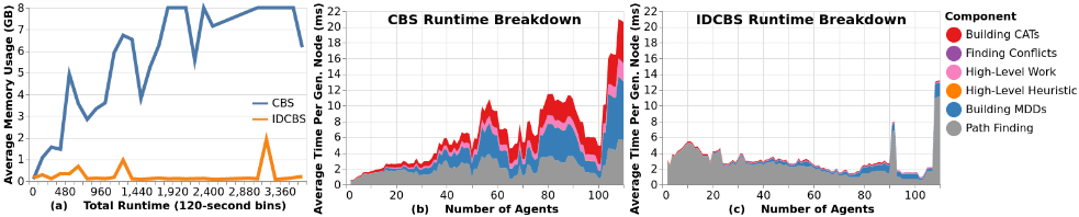
Figure 2(a) provides further insight. Here, we compare the average memory usage (out of 8GB available) for the two algorithms (y-axis) as a function of the CPU time required to solve the problem instance (in buckets of 2 minutes). As CBS runs longer, it needs more memory, while the memory needs of IDCBS remain relatively constant. In Section 4, we show how IDCBS can substantially shorten the CPU time per CT node versus CBS (see Figure 2(c)), which allows IDCBS to expand more CT nodes and find solutions faster. In Section 5, we show that IDCBS is in general much stronger than CBS.
4 Reducing the Time-Per-Node via DFS
A modern CBS implementation performs 6 main activities: (1) Finding low-level paths (Lines 4 and 35). (2) Building MDDs, which represent all possible paths of the same cost for an agent (Line 13). (3) Building the conflict avoidance table (CAT) [Standley, 2010] which tries to steer agents away from each other to avoid conflicts (Line 34). (4) Finding all new conflicts that were caused by the newly-planned paths in a CT node (Line 37). (5) Computing the h-value of a CT node (high-level heuristic) (Line 14). And, (6) other highlevel work, i.e., queuing and node construction operations to maintain OPEN (remaining lines).
Figure 2(b) shows the breakdown of the average time per generated CT node of CBS to these 6 components as the number of agents increases over all problem instances that were solved by both algorithms. Clearly, each of the components takes a measurable part of the time, with only computing the high-level heuristic (Component 5) and finding conflicts (Component 4) being substantially less time-consuming than the rest, for reasons described below.
Generating a node both under a best-first-search and under a depth-first search (DFS) is done in the context of the parent node. But there is a fundamental difference between best-first search and DFS. Best-first search jumps around the search tree. The internal information of a node is not passed between successive node expansions because nodes in different parts of the search space can be very different. Therefore, in best-first search each node typically holds all the necessary information in its own data structures. By contrast, DFS only moves between parent nodes and children (and back). So, a global current-node data structure can be maintained. When a node is generated, we calculate and store the difference ∆ between a parent and its child and undo this ∆ when backtracking. In the next subsections, we exploit this idea, and for each of the components, we introduce mechanisms that compute the ∆ from the parent node efficiently, mostly using incremental algorithms. Incremental algorithms use the work of previous executions to speed up solving a different but relatively similar problem instance.
Figure 2(c) shows the same breakdown for IDCBS with the incremental methods presented next and shows almost an order of magnitude reduction in CPU time per node. The incremental approaches have reduced all the components independently of each other as seen in the figure. We next cover each component in turn.
4.1 Component 1: Finding Low-Level Paths
A single constraint is added for one agent in every CT node. Consequently, the low-level path finding task is very similar to the last path-planning task for this agent that was performed in one of the ancestors of the CT node. Therefore, executing the low-level search from scratch might be wasteful. Instead, we can use incremental search algorithms; they use information from previous similar searches to speed up the new search. We use Lifelong Planning A* (LPA*) [Koenig et al., 2004] for the low-level search and provide a brief overview of LPA* next (see the original paper on LPA* for a full description).
LPA* is an incremental version of A*. LPA* is invoked again after vertices or edges are added to or deleted from the graph or the costs of some of the edges change. LPA* then replans a new path by using information from the previous executions, thereby significantly reducing the effort needed to plan from scratch. Like A*, LPA* maintains g(v) - the distance from start to each vertex v. LPA* also maintains the rhs-value of a vertex v (one-step lookahead values based on the g-values) to be the minimum of g(v′ ) + c(v′ , v) over all neighbours v′ of v. A vertex is called locally consistent iff its g-value equals its rhs-value. LPA* maintains a priority queue OPEN which always contains exactly the locally inconsistent vertices. LPA* expands the vertex with the lowest key in OPEN. The key k(v) of vertex v is a vector with two components: k(v) = [k1(v), k2(v)], where k1(v) = min(g(v), rhs(v)) + h(v) and k2(v) = min(g(v), rhs(v)) (g- and rhs-values that have not yet been computed are initialized to ∞). Keys are compared according to k1, and, in case of a tie, according to k2.
During it first execution, LPA* behaves like A*. A new execution is invoked after some changes to the underlying graph were made. In new executions, LPA* starts by first carrying over OPEN and CLOSED from the previous execution, including the g- and rhs-values. LPA* then updates the rhs-values of the vertices which are direct neighbors of the changed components (e.g., edges with updated costs). It also updates OPEN to reflect new locally consistent and inconsistent vertices from this set (which is a relatively cheap operation). Then, LPA* repeatedly expands vertices until the goal vertex is locally consistent and its key is smaller than the smallest key in OPEN. In this case, the g-value of the goal vertex is the cost of a shortest path from the start vertex to the goal. This allows LPA* to focus only on locally inconsistent vertices and it was shown that this can require less work than running A* from scratch on the changed graph.
Using LPA* for the Low Level of CBS
Adding a constraint 〈ai, v, t〉 to a CT node N can be viewed as deleting vertex vt from the TEG. Thus, the TEG of N is very similar to the previous TEG which was used the last time a path for ai was needed in an ancestor of N. This calls for using LPA* to search the new TEG instead of using A*. However, a fewmodifications are in order for this scenario.
(1) LPA* assumes a single goal vertex. For example, a typical path-finding execution terminates when the presumablyknown goal vertex is locally consistent and its key is smaller than the smallest key in OPEN. But, in a TEG, the goal location appears in many timesteps. To enable LPA* to search a TEG, we add a single vertex gfinal to the TEG that serves as LPA*'s single goal vertex. Each goal vertex gt in the TEG is connected with a zero-cost (dummy) edge to this new goal vertex. Luckily, the low-level heuristic only takes the location into account (the timestep is ignored), so it guides the search toward any goal vertex, regardless of its timestep.
(2) LPA* performs better when the changes in the graph occur closer to the goal vertex. LPA* re-expands a smaller subtree in this case [Koenig et al., 2004]. Therefore, as a tiebreaker (e.g., among cardinal conflicts), choose the closest conflict to the goal vertices of the conflicting agents.
(3) To make use of a CAT, LPA* keys need a third component k3(v), that represents the lowest number of conflicts of a shortest path for the given agent from start to v with the paths of other agents, as stored in the CAT. k3 is used in case there is a tie with respect to both k1 and k2.
Updating k3(v) for all vertices of the LPA* instances of all other agents each time the path of an agent is replanned would be too costly, because those LPA* instances would then have to propagate the cost changes down their trees. So, the k3(v) values are only updated lazily, when a vertex is modified for another reason. As a result, k3(v) may be out of date if the paths of other agents have changed since k3(v) was computed in a previous execution of LPA*. In this case, v has remained locally consistent since then, and k3(v) has not been recomputed. This can cause LPA* to find paths with new non-cardinal or semi-cardinal conflicts that could have been avoided if k3(v) had been fully up-to-date. 2
2 This only happens for LPA* because it reuses information. It would not happen for A* as it runs from scratch considering the current paths of the other agents.
This problem is mitigated by continuing the LPA* execution until all paths of the same cost are found and using the path with the smallest number of conflicts by consulting the CAT. However, this is only done when the CT node has no cardinal conflicts, because, when a cardinal conflict is resolved, other conflicts are likely to be indirectly resolved and this process would be redundant. An additional way to mitigate this problem is to use the Bypassing Conflicts (BP) enhancement [Boyarski et al., 2015a] (Lines 26-26 of Algorithm 1). BP resolves some non-cardinal or semi-cardinal conflicts without increasing the depth of the CT. When a child CT node is found to have the same sum of costs as its parent, and fewer conflicts, the replanned path is copied into the parent node, replacing the the path of the agent in the parent node. The updated parent node is then be re-inserted into OPEN, and the child node is discarded. BP is crucial in IDCBS because it further handles the issue of increased numbers of non-cardinal and semi-cardinal conflicts.
4.2 Component 2: BuildingMDDs
Recall that CBS builds MDDc i in the context of CT node N, taking the constraints on agent ai into account. Building MDDc i non-incrementally is implemented as a two-stage process with forward and backward searches. First, a forward A* search over the TEG is executed from start0i under the constraints that are imposed on agent ai. Backward MDD edges from each node back to all of its possible parents are constructed. This search does not stop when goalc i is expanded, but continues to expand all nodes v such that f(v) ≤ c and does not generate nodes v such that f(v) > c. At the end of this stage, we have generated all nodes v with f(v) ≤ c, even if they are not part of a path of cost c to the goal vertex. Such surplus nodes are pruned next. Second, a backward breadth-first search is performed over the nodes generated in the forward search. The search starts from goalc i and generates forward MDD edges to goalc i from all nodes vt for which (1) (v, goali) ∈ E and (2) t = c - 1. The search continues backward in this way until start0i is reached. All generated nodes that do not have forward edges (from the backward search) connected to them at the end of the backward search are repeatedly deleted, and the resulting doublyconnected structure is MDDc i .
Figures 1(c-e) show the stages of building an MDD of depth 4 for agent a1 from vertex S to vertex G on the graph in Figure 1(a). In this example, assume that another agent is planned to pass through ai's goal vertex, taking a unidirectional edge into vertex X2 from some other vertex in the graph (not in the figure), moving from X2 to G3 , and taking a unidirectional edge out of G3 and exiting the example. CBS has eventually added vertex constraints for a1 on X and timestep 2 and on G and timestep 3, and an edge constraint on moving in the opposite direction from G to X at timestep 2 (red crosses). Figure 1(c) shows all nodes that were generated at the end of the first stage. Figure 1(d) shows the result of the second stage. Figure 1(e) shows the MDD that resulted from pruning all nodes that do not lead to G41 (i.e., G21 ).
This two-phase process is relatively time-consuming. It is especially problematic when CBS uses a high-level heuristic, because MDDs are needed for every agent that has a vertex in the conflict graph (see below). Moreover, when a new MDD is needed due to new constraints, CBS builds it from scratch. IDCBS mitigates this issue as follows. When using LPA* for the low-level search, the MDD can be quickly constructed. Every time LPA* halts with a new path, for every node v with k(v) < k(goal), g(v) is equal to the true distance from the start vertex to v. So, when a new MDD is needed, IDCBS resumes the LPA* execution for agent ai, now expanding all nodes v with k(v) = k(goal) and finishing the forward search part of building the MDD with very little effort. IDCBS then performs a similar backward search to complete the MDD. Thus, not only is most of the forward search effort saved, but also the pruning effort in the backward search, because LPA* keeps all nodes for its next execution.
4.3 Component 3: Building the CAT
Consider a CT node where a path for agent ai is needed by CBS. A Conflict-Avoidance Table (CAT) [Standley, 2010] holds the location-time pairs that make up the paths of all other agents in the CT node. While replanning a path for agent ai, the low level of CBS uses the CAT to break ties among paths of the same cost in favor of paths that cause fewer conflicts with the current paths of the other agents as given by the CAT. Because the size of the CAT is relatively large, it is usually built from scratch for every new CT node, mainly to save memory (Line 34 in Algorithm 1).
In IDCBS, instead of building the CAT from scratch each time a low-level search is invoked, a single global CAT is maintained. This table holds location-time pairs of the paths of all agents in the current CT node. The CAT is initialized with the paths in the root node of the CT. Every time a CAT is needed, the path that is going to be replanned is removed from the CAT. Then, when the low-level search finishes, the newly-planned path is incorporated into the CAT and the DFS continues. When the DFS backtracks, the same is done in reverse. Thus, for a problem instance with k agents, one path is removed from the CAT once and inserted into it once, instead of k paths being inserted into a newly generated CAT for each new CT node.
4.4 Component 4: Finding NewConflicts
Since in both best-first search and DFS traversals, the child CT node is constructed from its parent, some parts of CBS are typically already implemented in an incremental way. When a new CT node is generated, only the newly-planned paths are checked for conflicts with all other paths. The conflicts between the paths that remain unchanged are carried over from the new parent of the new node.
4.5 Component 5: Computing The Heuristic
For each CT node N, the size of the minimum vertex cover (MVC) of a corresponding cardinal-conflict graph is used as an admissible h-value for the remaining cost to reach a goal CT node in the subtree rooted at N [Felner et al., 2018]. The h-value of the root node is computed from scratch. Children of a CT node with an MVC of size k only need to check whether their MVC is of size k - 1 and possibly also k. Otherwise, it is k + 1 [Felner et al., 2018]. We tried a different approach of using a Mixed Integer Programming (MIP)
| #agents | 10 | 20 | 30 | 40 | 50 | 70 | 90 |
|---|---|---|---|---|---|---|---|
| #instances | 62 | 55 | 44 | 37 | 27 | 13 | 9 |
| Average | Number | of | Generated | Nodes | (in 1000x) | ||
| CBS | 6.2 | 33.0 | 22.5 | 16.0 | 7.4 | 18.2 | 4.8 |
| IDCBS | 17.9 | 9.1 | 15.8 | 14.3 | 14.1 | 223.4 | 2.6 |
model to directly compute the MVC. Modern MIP solvers reuse information from previous computations. We exploited this property by maintaining the same MIP model and adding or removing edges from the cardinal conflict graph as needed, which sped up the execution. We used Gurobi Optimizer as the MIP solver. It turned out that this is far faster than the previous approach, so we use it for both CBS and IDCBS throughout our experimentation.
4.6 Component 6: High-Level Work
Maintaining a stack is cheaper than maintaining a priority queue, so this runtime activity is also faster in IDCBS.
5 Experimental Results
All experiments were run on a Linux laptop with an Intel Core i7-8650U CPU running at 1.9GHz. CBS and IDCBS were implemented in the same C++ code base.
To compare CBS and IDCBS, we experimented on the MAPF benchmark [Stern et al., 2019], which contains 32 grids with different attributes (city maps, grids with random obstacles, mazes, warehouse maps, etc.), each with a number of scenarios (i.e., start and goal locations for up to 7,000 agents). We increased the number of agents on the first scenario of each grid for each algorithm until we reached the runtime limit (1 hour) or memory limit (8GB). For higher numbers of agents the outcome of the algorithm was considered an implicit fail.
Table 1 (page 3) shows the number of solved problem instances and number of different failures for CBS and IDCBS. Out of 3380 problem instances, 190 were solved by IDCBS but not by CBS, 45 were solved only by CBS and not by IDCBS, and 64 were not solved by either algorithm. This difference is statistically significant (McNemar's Test produces χ2 = 89.5).
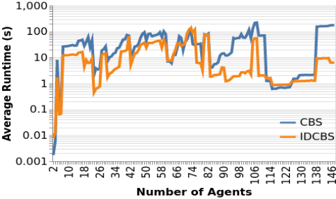
To the best of our knowledge, these 190 problem instances have never been solved optimally before. Table 2 compares the average number of nodes generated by CBS and IDCBS. Similarly to IDA*, on exactly the same CT, IDCBS generates more CT nodes than CBS. In practice, however, IDCBS generated fewer CT nodes than CBS in some cases because IDCBS uses different low-level path finding (A* versus LPA*) and chooses conflicts differently. So, their CTs can be different. Figure 3 shows the average runtime over all problem instances that were solved by both CBS and IDCBS on a logarithmic scale. IDCBS outperforms CBS in its CPU time by up to two orders of magnitude.
6 Summary and Conclusions
CBS is a memory-intensive algorithm since its implementations typically store a significant amount of information for each CT node in its search frontier. This has gone largely unnoticed since the practice has been to run CBS for very short time limits only. In this work, we have presented a memoryefficient version of CBS using iterative deepening and incremental algorithms to update data.
There is a huge scope for future work. In particular, we need to compare different types of traversals of the CT: for example, to discover when iterative deepening depth-first search is preferable to best-first search and to experiment with other traversals, such as depth-first branch and bound. Also, since we made the exploration of CT nodes significantly cheaper for IDCBS than for CBS, we need to re-visit many of the design choices of CBS that were handled in this paper. We should investigate how incremental data structures affect other CBS variants, such as ECBS [Barer et al., 2014], Lazy CBS [Gange et al., 2019], CBS with Priorities (CBSwP) and Priority-Based Search (PBS) [Ma et al., 2019].
Building efficient implementations of CBS and IDCBS is a substantial undertaking of algorithmic engineering, as described in this paper. The code is available on the mapf.info website and at https://github.com/eli-b/idcbs.
Acknowledgements
The research at Ben-Gurion University of the Negev was supported by the Israel Ministry of Science, ISF grant 844/17 and BSF grant 2017692. The research at the University of Southern California was supported by NSF grants 1409987, 1724392, 1817189, 1837779 and 1935712, as well as a gift from Amazon.
@inproceedings{ijcai2020p565,
  title     = {Iterative-Deepening Conflict-Based Search},
  author    = {Boyarski, Eli and Felner, Ariel and Harabor, Daniel and Stuckey, Peter J. and Cohen, Liron and Li, Jiaoyang and Koenig, Sven},
  booktitle = {Proceedings of the Twenty-Ninth International Joint Conference on
               Artificial Intelligence, {IJCAI-20}},
  publisher = {International Joint Conferences on Artificial Intelligence Organization},
  editor    = {Christian Bessiere},
  pages     = {4084--4090},
  year      = {2020},
  month     = {7},
  note      = {Main track},
  doi       = {10.24963/ijcai.2020/565},
  url       = {https://doi.org/10.24963/ijcai.2020/565},
}
TY - CPAPER TI - Iterative-Deepening Conflict-Based Search AU - Boyarski, Eli AU - Felner, Ariel AU - Harabor, Daniel AU - Stuckey, Peter J. AU - Cohen, Liron AU - Li, Jiaoyang AU - Koenig, Sven T2 - Proceedings of the Twenty-Ninth International Joint Conference on Artificial Intelligence, IJCAI-20 PB - International Joint Conferences on Artificial Intelligence Organization PY - 2020 SP - 4084 EP - 4090 DO - 10.24963/ijcai.2020/565 UR - https://doi.org/10.24963/ijcai.2020/565 ER -Copied
Machine-readable versions of this paper, for tools and AI agents:





