
Adaptive Edge Attention for Graph Matching with Outliers
Proceedings of the Thirtieth International Joint Conference on Artificial Intelligence. Main Track. Pages 966-972.
https://doi.org/10.24963/ijcai.2021/134
Keywords
- Computer Vision: Recognition: Detection, Categorization, Indexing, Matching, Retrieval, Semantic Interpretation
- Machine Learning: Deep Learning
Abstract
Graph matching aims at establishing correspondence between node sets of given graphs while keeping the consistency between their edge sets. However, outliers in practical scenarios and equivalent learning of edge representations in deep learning methods are still challenging. To address these issues, we present an Edge Attention-adaptive Graph Matching (EAGM) network and a novel description of edge features. EAGM transforms the matching relation between two graphs into a node and edge classification problem over their assignment graph. To explore the potential of edges, EAGM learns edge attention on the assignment graph to 1) reveal the impact of each edge on graph matching, as well as 2) adjust the learning of edge representations adaptively. To alleviate issues caused by the outliers, we describe an edge by aggregating the semantic information over the space spanned by the edge. Such rich information provides clear distinctions between different edges (e.g., inlier-inlier edges vs. inlier-outlier edges), which further distinguishes outliers in the view of their associated edges. Extensive experiments demonstrate that EAGM achieves promising matching quality compared with state-of-the-arts, on cases both with and without outliers. Our source code along with the experiments is available at https://github.com/bestwei/EAGM.
- [Bourdev and Malik, 2009] Lubomir Bourdev and Jitendra Malik. Poselets: Body part detectors trained using 3d hu- man pose annotations. In ICCV, pages 1365-1372, 2009.
- [Bresenham, 1965] Jack E Bresenham. Algorithm for com- puter control of a digital plotter. IBM Systems Journal, 4(1):25-30, 1965.
- [Caetano et al., 2006] Tiberio S Caetano, Terry Caelli, Dale Schuurmans, and Dante Augusto Couto Barone. Graphical models and point pattern matching. IEEE Trans. Pattern Anal. Mach. Intell., 28(10):1646-1663, 2006.
- [Caetano et al., 2009] Tibério S Caetano, Julian J McAuley, Li Cheng, Quoc V Le, and Alex J Smola. Learning graph matching. IEEE Trans. Pattern Anal. Mach. Intell., 31(6):1048-1058, 2009.
- [Cho et al., 2010] Minsu Cho, Jungmin Lee, and Ky- oung Mu Lee. Reweighted random walks for graph match- ing. In ECCV, pages 492-505, 2010.
- [Cho et al., 2013] Minsu Cho, Karteek Alahari, and Jean Ponce. Learning graphs to match. In ICCV, pages 25-32, 2013.
- [Cignoni et al., 1998] Paolo Cignoni, Claudio Montani, and Roberto Scopigno. Dewall: A fast divide and conquer de- launay triangulation algorithm in ed. Computer-Aided De- sign, 30(5):333-341, 1998.
- [Deng et al., 2009] Jia Deng, Wei Dong, Richard Socher, Li- Jia Li, Kai Li, and Li Fei-Fei. Imagenet: A large-scale hierarchical image database. In CVPR, pages 248-255, 2009.
- [Egozi et al., 2012] Amir Egozi, Yosi Keller, and Hugo Guterman. A probabilistic approach to spectral graph matching. IEEE Trans. Pattern Anal. Mach. Intell., 35(1):18-27, 2012.
- [Everingham et al., 2010] Mark Everingham, Luc Van Gool, Christopher KI Williams, John Winn, and Andrew Zisser- man. The pascal visual object classes (voc) challenge. In- ternational Journal of Computer Vision, 88(2):303-338, 2010.
- [Gold and Rangarajan, 1996] Steven Gold and Anand Ran- garajan. A graduated assignment algorithm for graph matching. IEEE Trans. Pattern Anal. Mach. Intell., 18(4):377-388, 1996.
- [Kingma and Ba, 2015] Diederik P Kingma and Jimmy Ba. Adam: A method for stochastic optimization. In ICLR, 2015.
- [Leordeanu and Hebert, 2005] Marius Leordeanu and Mar- tial Hebert. A spectral technique for correspondence prob- lems using pairwise constraints. In ICCV, pages 1482- 1489, 2005.
- [Leordeanu et al., 2009] Marius Leordeanu, Martial Hebert, and Rahul Sukthankar. An integer projected fixed point method for graph matching and map inference. In NIPS, pages 1114-1122, 2009.
- [Leordeanu et al., 2011] Marius Leordeanu, Andrei Zanfir, and Cristian Sminchisescu. Semi-supervised learning and optimization for hypergraph matching. In ICCV, pages 2274-2281, 2011.
- [Leordeanu et al., 2012] Marius Leordeanu, Rahul Suk- thankar, and Martial Hebert. Unsupervised learning for graph matching. International Journal of Computer Vi- sion, 96(1):28-45, 2012.
- [Liu and Qiao, 2013] Zhi-Yong Liu and Hong Qiao. Gnccp-graduated nonconvexityand concavity procedure. IEEE Trans. Pattern Anal. Mach. Intell., 36(6):1258- 1267, 2013.
- [Loiola et al., 2007] Eliane Maria Loiola, Nair Maria Maia de Abreu, Paulo Oswaldo Boaventura-Netto, Peter Hahn, and Tania Querido. A survey for the quadratic assignment problem. European Journal of Operational Research, 176(2):657-690, 2007.
- [Simonyan and Zisserman, 2014] Karen Simonyan and An- drew Zisserman. Very deep convolutional networks for large-scale image recognition. arXiv preprint arXiv:1409.1556, 2014.
- [Torresani et al., 2008] Lorenzo Torresani, Vladimir Kol- mogorov, and Carsten Rother. Feature correspondence via graph matching: Models and global optimization. In ECCV, pages 596-609, 2008.
- [Wang et al., 2018] Tao Wang, Haibin Ling, Congyan Lang, and Songhe Feng. Graph matching with adaptive and branching path following. IEEE Trans. Pattern Anal. Mach. Intell., 40(12):2853-2867, 2018.
- [Wang et al., 2019] Runzhong Wang, Junchi Yan, and Xi- aokang Yang. Learning combinatorial embedding net- works for deep graph matching. In ICCV, pages 3056- 3065, 2019.
- [Wang et al., 2020] Tao Wang, He Liu, Yidong Li, Yi Jin, Xiaohui Hou, and Haibin Ling. Learning combinatorial solver for graph matching. In CVPR, pages 7568-7577, 2020.
- [Yan et al., 2020] Junchi Yan, Shuang Yang, and Edwin R Hancock. Learning for graph matching and related com- binatorial optimization problems. In IJCAI, 2020. IJCAI
- [Yu et al., 2020a] Tianshu Yu, Runzhong Wang, Junchi Yan, and Baoxin Li. Learning deep graph matching with channel-independent embedding and hungarian attention. In ICLR, 2020.
- [Yu et al., 2020b] Tianshu Yu, Junchi Yan, and Baoxin Li. Determinant regularization for gradient-efficient graph matching. In CVPR, pages 7123-7132, 2020.
- [Zanfir and Sminchisescu, 2018] Andrei Zanfir and Cristian Sminchisescu. Deep learning of graph matching. In CVPR, pages 2684-2693, 2018.
- [Zhou and De la Torre, 2012] Feng Zhou and Fernando De la Torre. Factorized graph matching. In CVPR, pages 127-134, 2012.
References were extracted automatically from the PDF and may contain errors.
Full text extracted automatically from the PDF; figures, tables and equations may differ. The PDF is the version of record.
1 Introduction
Aiming at establishing node correspondence between graphs while keeping the consistency between their edges, graph matching has been widely applied in computer vision, e.g., shape matching, object recognition, and tracking, etc. From finding node correspondence in pure cases (i.e., all nodes are inliers), to establishing matches between inliers while overcoming interference caused by outliers, there are many open issues to be solved in this field. Actually, the outliers are common in practical scenarios. In this paper, we focus on addressing the general graph matching problem with outliers.
∗Contact Author
As a classical combinatorial optimization problem, graph matching is NP-hard and generally solved by acceptable suboptimal solutions. Early methods [Gold and Rangarajan, 1996; Leordeanu et al., 2009; Cho et al., 2010; Egozi et al., 2012; Liu and Qiao, 2013] propose approximate algorithms with some relaxations. Then machine learning methods [Torresani et al., 2008; Caetano et al., 2009; Leordeanu et al., 2011; Leordeanu et al., 2012; Cho et al., 2013] compute node and edge affinities by simple and shallow parametric models, while the accuracy promotion is limited. Recently, encouraged by the successes of deep neural networks in many research areas, deep learning methods [Zanfir and Sminchisescu, 2018; Wang et al., 2019; Yu et al., 2020a; Wang et al., 2020] are introduced for learning the combinatorial solver in graph neural networks (GNN). Point positions and object appearance in visual matching tasks provide rich geometric and semantic features for these methods. However, two important challenges remain unsolved.
First, the outliers bring inevitable interference to the matching process in practical scenarios. Previous methods usually propose enhanced node features to reduce interference of outliers, but devote insufficient discrimination on the features of associated edges. Second, the initial graph structure in visual matching tasks is generally constructed in heuristic ways (e.g., Delauney triangulation or k-nearest), and the obtained edges are all utilized during the learning process. Some edges thus generated are necessary, but others may be noisy. In fact, the impact of each edge on graph matching is different. Besides, different from links in social networks and bonds in molecular graphs, features of these edges are typically constructed by simple combinations (e.g., concatenation or element-wise multiplication) over features from their associated nodes. Thus reasonable and informative descriptions of edges are worth exploring.
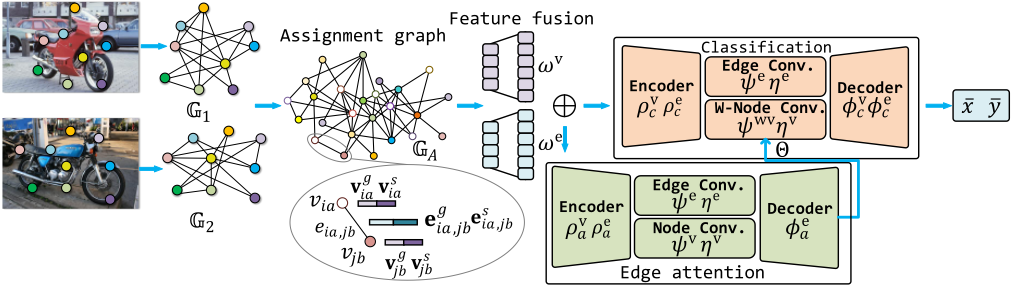
To address the two challenges mentioned above, we propose an Edge Attention-adaptive Graph Matching (EAGM) network (as illustrated in Figure 1), and a novel descriptive approach of edge features. Given a pair of graphs to be matched, EAGM transforms the matching between them into a node and edge classification problem over their assignment graph. The geometric features and semantic features of the assignment graph are fused to encode jointly position and appearance information. Then EAGM learns the edge attention on the assignment graph with fused features, which indicates the impact of each edge on graph matching. The edge attention is imposed into the learning of node and edge classification on the assignment graph, which adjusts the learning of edge representations adaptively. The final predicted labels indicate whether the two original nodes or edges are matched in the graph matching problem.
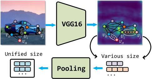
To alleviate the interference caused by outliers, we design the edge semantic features to distinguish outliers from the aspect of their adjacent edges, rather than enhancing the node features only. We consider each edge as consisting of discrete points, i.e., its passing pixel points in visual matching tasks. Then we describe its semantic features by involving the convolutional features of all passed pixel points. Compared with the previous approaches relying on features of the associated nodes, such edge features are more informative and independent. It can provide strong distinctions between inlier-inlier and inlier-outlier edges. Since the information of associated nodes is also included, the differences between the two kinds of edges further enhance the discrimination between inliers and outliers.
In summary, the main contributions of this paper include:
- We propose an Edge Attention-adaptive Graph Matching network, EAGM, which adjusts edge attention adaptively during learning graph matching. The impact of each edge on graph matching is described by the learned edge attention. The final predicted node and edge labels of the assignment graph indicate the matching relations between the two original graphs.
- We devise a novel edge feature by encoding semanticaware information distributed spatially around edge pixels. Such feature not only provides reasonable and independent description for edges in visual matching tasks, but also distinguishes outliers by their adjacent edges.
- EAGM achieves promising performance on three popular benchmarks, on experiments both with and without outliers.
2 RelatedWork
Graph matching has received significant attention in decades. Readers are referred to [Yan et al., 2020] for a comprehensive acquaintance. Early methods [Gold and Rangarajan, 1996; Leordeanu et al., 2009; Cho et al., 2010; Egozi et al., 2012; Zhou and De la Torre, 2012; Liu and Qiao, 2013; Wang et al., 2018] usually search acceptable sub-optimal solutions via heuristics. [Leordeanu et al., 2009] utilizes original discrete constraints to optimize graph matching with climbing and convergence properties. Recently, [Yu et al., 2020b] proposes a determinant regularization technique on the correspondence matrix to perform gradient-efficient continuation optimization. However, being limited by handcrafted affinities, these methods still lack robust ability on real-work matching tasks.
Inspired by growing data and features, some methods [Torresani et al., 2008; Caetano et al., 2009; Leordeanu et al., 2011; Leordeanu et al., 2012; Cho et al., 2013] devote attention to learn parameters of the corresponding affinity matrix, rather than the handcrafted affinities. [Cho et al., 2013] utilizes structured SVM to parameterize a graph model, and apply its structural attributes to visual matching. Weight parameters can also be learned via semi-supervised [Leordeanu et al., 2011] or unsupervised [Leordeanu et al., 2012] models. Although the affinity weights are learnable, the node representations and structural information are still to be mined.
Recent deep learning methods [Zanfir and Sminchisescu, 2018; Wang et al., 2019; Yu et al., 2020a; Wang et al., 2020] utilize features extracted by convolutional neural networks (CNN) or geometric information to initialize graph features, and learn a combinatorial solver by GNN. The pioneer work [Zanfir and Sminchisescu, 2018] computes unary and pairwise node affinities by CNN features, and adopts spectral matching [Leordeanu and Hebert, 2005] as a differentiable (but fixed) combinatorial solver. [Wang et al., 2019] adopts GNN to aggregate graph structure information into node representations, and a Sinkhorn net is introduced as the combinatorial solver on node affinities. [Yu et al., 2020a] devises a channel-independent embedding method, and utilizes Hungarian attention to smooth objective learning for graph matching. [Wang et al., 2020] converts matching between two graphs into a node classification problem in their assignment graph, and learns the affinity functions and combinatorial solver simultaneously.
Despite the satisfactory progress achieved, the above methods are still sensitive to common outliers in practical scenarios, or lack impact adjustment of each edge on graph matching. In this paper, we overcome these problems by learning the edge attention-adaptive graph matching and by designing a novel edge semantic description.
3 Definition of GraphMatching
An undirected graph is represented by G = (V, E, V, E),
- V = {v1, . . . , vn} denotes the node set, |V| = n,
- E ⊆ V×V denotes the edge set, |E| = m,
- V = {vi|vi ∈ Rdv , i = 1, . . . , n} denotes the node feature set,
- E = {ei|ei ∈ Rde , i = 1, . . . ,m} denotes the edge feature set.
Given two graphs G1 = (V1, E1, V1, E1) and G2 = (V2, E2, V2, E2) with 1 |V1| = |V2| = n, the graph matching problem is to find a node correspondence X ∈ {0, 1}n×n between G1 and G2. Xia = 1 iff vi ∈ V1 corresponds to va ∈ V2. Graph matching is generally formulated by a quadratic assignment programming (QAP) problem [Loiola et al., 2007].
The vector x∗ denotes the desired node correspondence. The required one-to-one constraint is described by X1n = 1n and X⊤1n = 1n ( 1n denotes a vector of n ones). K ∈ Rn2×n2 is the corresponding affinity matrix,
1 We assume the two graphs have the same size n, and definitions can be extended to varied sizes, e.g., by adding dummy nodes.
where A ∈ Rn×n is a symmetric adjacency matrix describing node connections, and Aij = 1 iff there is an edge ei,j = (vi, vj) ∈ E. svia measures the affinity between the node features vi ∈ V1 and va ∈ V2. seiajb measures the affinity between edge features ei,j ∈ E1 and ea,b ∈ E2.
4 Edge Attention-Adaptive GraphMatching
In the proposed EAGM (Figure 1), graph matching is learned by four modules:
- Edge Semantic Description. This module classifies node and edge features of the two given graphs G1 and G2 into the geometric features and the semantic features. The edge semantic features are designed emphatically.
- Assignment Graph Generation. This module generates the assignment graph GA for G1 and G2, and fuses its geometric features and semantic features. The original graph matching between G1 and G2 is converted into the node and edge binary classification in GA.
- Edge Attention. The edge attention module is the core component of EAGM. It takes GA with fused features as input, and learns the attention for each edge of GA to adjust its impact on learning graph matching. This module adopts an encoder-decoder architecture, along with a convolution sub-module. The coupled encoder and decoder sub-modules transform fused features of GA into latent representations, and predict the edge attention Θ based on the final graph state, respectively. The convolution sub-module consists of l1 coupled edge convolution layers and node convolution layers, which learns node and edge representations for learning attention Θ.
- Classification. This module combines GA with fused features and the edge attention Θ, and predicts final node and edge labels. It has similar autoencoder architecture with the former module. Its decoder outputs the predicted node and edge labels. The convolution submodule consists of l2 coupled edge convolution layers and weighted-node convolution layers, and utilizes the
edge attention Θ to parameterize the aggregation in the weighted-node convolution layers. Besides, we propose a binary cross-entropy loss for guiding learning of edge representations and edge attention.
4.1 Edge Semantic Description
We categorize the node and edge features into two types, geometric feature and semantic feature,
- V = {V g , V s }, V g = {vg i |vg i ∈ Rdgv, i = 1, . . . , n} and V s = {vs i |vs i ∈ Rdsv , i = 1, . . . , n} denote the node geometric and semantic feature set, respectively,
- E = {E g , E s }, E g = {egi |egi ∈ Rdge , i = 1, . . . ,m} and E s = {esi |esi ∈ Rdse , i = 1, . . . ,m} denote the edge geometric and semantic feature set, respectively.
Specifically, we utilize the 2D Cartesian coordinates of each node vi as its geometric feature vg i = [xi, yi], and concatenate the geometric features of head node vhi and tail node vti associated with each edge ei to form its geometric feature egi = [vghi ; vg ti ].
For the node semantic feature, we extracted CNN feature maps from the input images, and interpolate them as the size of images. The spatially corresponding feature vector located at (xi, yi) for each node is selected as its semantic feature vs i ∈ Rdsv . The node semantic features are L2 normalized.
To clearly explain the design of edge semantic feature, we take an edge ei,j = (vi, vj) in Figure 2 as an example. We firstly adopt Bresenham's line algorithm [Bresenham, 1965] to compute the pixel points passed by the edge ei,j, and collect them as a point set P = {vi, p1, . . . , pk, vj}. Then the semantic features of these points are constructed by the above operations of node semantic features, and form a feature set V s P = {vs i |vs i ∈ Rdsv, i = 1, . . . , k + 2}. Next we stack these features, and obtain the initial edge semantic feature esi,j ∈ Rk×dsv . Notably, different edges pass different amounts of pixel points (e.g., ei,j and ea,b), but the size of all edge features should be unified in a GNN. Thus we finally adopt the max pooling operation on the initial edge semantic features to obtain the unified size dse , e.g., esi,j ∈ Rdse . The edge semantic features are also L2 normalized.
4.2 Assignment Graph Generation
Inspired by the successful assignment graph in [Leordeanu and Hebert, 2005; Cho et al., 2010; Wang et al., 2020], we transform the graph matching problem between the two graphs G1 and G2 into a node and edge binary classification problem in the assignment graph GA = (VA, EA, VA, EA). GA describes all candidate node and edge correspondences between G1 and G2. For structure generation of GA, each candidate node correspondence vi ∈ V1 and va ∈ V2 generates a node via ∈ VA. An edge eia,jb = (via, vjb) ∈ EA is constructed iff there are two edges ei,j ∈ E1 and ea,b ∈ E2.
For feature initialization of GA, we concatenate the initial geometric and semantic features of G1 and G2 respectively.
To enable the following modules to learn about both position and appearance jointly, we further fuse the geometric and semantic features of GA by two multilayer perceptrons (MLPs) ωv and ωe . They embed a node geometric feature and an edge geometric feature into their semantic features respectively:
where ωv (V gA) and ωe (E gA) denote the embedded node geometric features and edge geometric features, by applying ωv and ωe to each node and each edge respectively. Then the updated graph GA with fused features is passed to the following edge attention module and classification module as input.
Therefore, the original graph matching between G1 and G2 is converted into the binary classification problem in GA, i.e., positive and negatives nodes or edges are equivalent to the two original nodes or edges being matched or not.
4.3 Edge Attention Learning
The edge attention module takes the updated graph GA with fused features as input, and learns the attention θi of each edge ei ∈ EA for graph matching. It consists of three submodules, encoder, convolution, and decoder sub-module.
The encoder sub-module embeds the fused features VA and EA into latent representations by two MLPs ρva and ρea , respectively. The updated graph GA = (VA, EA, ρva (VA), ρea (EA)) is fed into the following convolution sub-module.
The convolution sub-module consists of l1 coupled edge convolution layers and node convolution layers, which updates latent representations of GA. Overall, the edge convolution layer aggregates the representations of the two associated nodes of each edge to update the representation of this edge. The following node convolution layer aggregates the representations of all the edges adjacent to each node to update the node representation.
Edge convolution. The edge convolution layer updates the edge representations of GA by firstly aggregating the representations vhi and vti of head and tail nodes of each edge ei ∈ EA to produce an intermediate edge representation ˆei.
where the operation ◦ denotes the Hadamard product between two vectors. Then the edge representation is updated by transforming the concatenation of the aggregated representation ˆ ei and the original edge representation ei.
Node convolution. The node convolution layer updates the node representations of GA by firstly aggregating the representations of associated edges E iA for each node vi ∈ VA to generate an intermediate node representation ˆvi.
Then the node representation is updated by a similar way in the edge convolution layer.
The three functions ψe , ηe , and ηv are implemented by MLPs.
The decoder sub-module predicts the edge attention Θ by the final graph state to indicate the impact of each edge on graph matching. Since we focus on learning attention for edges, this sub-module is implemented by only one MLP φea .
4.4 Classification
The classification module accepts GA with fused features and the learned edge attention Θ as input, and predicts node and edge labels of GA to reason whether the two original nodes and edges are matched respectively. The edge attention Θ is imposed into the learning of edge representations. This module has three similar sub-modules with the edge attention module. The encoder also embeds fused features of GA into latent representations by two MLPs ρvc and ρec respectively.
The convolution sub-module consists of l2 coupled edge convolution layers and weighted-node convolution layers.
Weighted-Node convolution. Different from the node convolution layer in the edge attention module, the aggregation in the weighted-node convolution layer is parameterized by the attention of associated edges Θi for each node vi ∈ VA.
| Method | aero | bike | bird | boat | bottle | bus | car | cat | chair | cow | d.table | dog | horse | m.bike | person | plant | sheep | sofa | train | tv | Avg. |
|---|---|---|---|---|---|---|---|---|---|---|---|---|---|---|---|---|---|---|---|---|---|
| IPFP | 25.1 | 26.4 | 41.4 | 50.3 | 43.0 | 32.9 | 37.3 | 32.5 | 33.6 | 28.2 | 26.9 | 26.1 | 29.9 | 32.0 | 28.8 | 62.9 | 28.2 | 69.3 | 33.8 | 36.6 | |
| RRWM | 30.9 | 40.0 | 46.4 | 54.1 | 52.3 | 35.6 | 47.4 | 37.3 | 36.3 | 34.1 | 28.8 | 35.0 | 39.1 | 36.2 | 39.5 | 67.8 | 38.6 | 45.0 49.4 | 70.5 | 41.3 | 43.0 |
| PSM | 32.6 | 37.5 | 49.9 | 53.2 | 47.8 | 34.6 | 50.1 | 35.5 | 37.2 | 36.3 | 23.1 | 32.7 | 42.4 | 37.1 | 38.5 | 62.3 | 41.7 | 54.3 | 72.6 | 40.8 | 43.1 |
| GNCCP | 28.9 | 37.1 | 46.2 | 53.1 | 48.0 | 36.3 | 45.5 | 34.7 | 36.3 | 34.2 | 25.2 | 35.3 | 39.8 | 39.6 | 40.7 | 61.9 | 37.4 | 50.5 | 67.0 | 34.8 | 41.6 |
| ABPF | 30.9 | 40.4 | 47.3 | 54.5 | 50.8 | 35.1 | 46.7 | 36.3 | 40.9 | 38.9 | 16.3 | 34.8 | 39.8 | 39.6 | 39.3 | 63.2 | 37.9 | 50.2 | 70.5 | 41.3 | 42.7 |
| GMN | 31.9 | 47.2 | 51.9 | 40.8 | 68.7 | 72.2 | 53.6 | 52.8 | 34.6 | 48.6 | 72.3 | 47.7 | 54.8 | 51.0 | 38.6 | 75.1 | 49.5 | 45.0 | 83.0 | 86.3 | 55.3 |
| PCA | 40.9 | 55.0 | 65.8 | 47.9 | 76.9 | 77.9 | 63.5 | 67.4 | 33.7 | 65.5 | 63.6 | 61.3 | 68.9 | 62.8 | 44.9 | 77.5 | 67.4 | 57.5 | 86.7 | 90.9 | 63.8 |
| CIE | 51.2 | 69.2 | 70.1 | 55.0 | 82.8 | 72.8 | 69.0 | 74.2 | 39.6 | 68.8 | 71.8 | 70.0 | 71.8 | 66.8 | 44.8 | 85.2 | 69.9 | 65.4 | 85.2 | 92.4 | 68.9 |
| LCSGM | 46.9 | 58.0 | 63.6 | 69.9 | 87.8 | 79.8 | 71.8 | 60.3 | 44.8 | 64.3 | 79.4 | 57.5 | 64.4 | 57.6 | 52.4 | 96.1 | 62.9 | 65.8 | 94.4 | 92.0 | 68.5 |
| EAGM | 49.4 | 62.1 | 64.6 | 75.3 | 90.9 | 80.9 | 71.1 | 61.3 | 48.7 | 65.9 | 87.5 | 58.4 | 66.3 | 60.1 | 56.3 | 97.1 | 64.7 | 60.6 | 96.0 | 93.0 | 70.5 |
To learn the more effective intermediate node representation ˆvi, the edge attention Θi adjusts the learning of edge representations E iA adaptively.
The decoder predicts the node labels ¯x and edge labels ¯y by the final graph state, and is implemented by two MLPs φvc and φec .
4.5 Loss
The ground-truth node-to-node and edge-to-edge correspondences are utilized to guide the training of our EAGM. We firstly define that the two edges ei ∈ E1 and ea ∈ E2 are matched iff their associated node pairs (vhi , vha ) and (vti , vta ) are matched respectively. Then we build the ground-truth edge-to-edge correspondence matrix Y ∈ {0, 1}m1×m2 between G1 and G2, where each element Yia = 1 iff ei ∈ E1 corresponds to ea ∈ E2.
To guide the learning of edge representations and edge attention, we measure a binary cross-entropy loss Le between the predicted edge labels ¯y and the ground-truth edge binary labels y = vec(Y) ∈ {0, 1}m1m2 .
Besides, we compute the binary cross-entropy loss Lv between the predicted node labels ¯x and the ground-truth node labels x, and the one-to-one matching constraint loss Lc,
where B ∈ {0, 1}2n×n2 is an auxiliary matrix, and ¯z ∈ {0, 1}n2 is an index vector (please refer to [Wang et al., 2020] for the details of Lv and Lc).
Finally, we combine the three losses to jointly guide the training of our EAGM,
where λe, λc ≥ 0 control the relative importance of Le and Lc respectively.
5 Experiments
5.1 Implementation &Evaluation Benchmarks
In our implementation, we build up our EAGM based on the state-of-the-art method [Wang et al., 2020], which learns
affinities and the combinatorial solver simultaneously. For all experiments, optimization is achieved via ADAM optimizer [Kingma and Ba, 2015] with initial learning rate 1 × 10⁻³ , and exponential decaying 2% per 2000 iterations. The CNN features in Sec. 4.1 are the concatenated feature maps of relu4 2 and relu5 1 of a VGG16 [Simonyan and Zisserman, 2014] network pre-trained on ImageNet [Deng et al., 2009]. We empirically set the number of convolutional layers l1 = 3 and l2 = 10 in the edge attention module and classification module respectively. The weights in Eq. 12 are set as λe = λc = 0.1 during training. All experiments are run on a single GTX-1080Ti GPU, and around 25 image pairs are processed per second.
Our EAGM is compared with the state-of-the-arts, including IPFP [Leordeanu et al., 2009], RRWM [Cho et al., 2010], PSM [Egozi et al., 2012], GNCCP [Liu and Qiao, 2013], ABPF [Wang et al., 2018], HARG [Cho et al., 2013], DetGM [Yu et al., 2020b], GMN [Zanfir and Sminchisescu, 2018], PCA [Wang et al., 2019], CIE [Yu et al., 2020a], and LCSGM [Wang et al., 2020] (the last four are deep learning methods). The experiments are performed on two cases with and without outliers, including three benchmarks for keypoint matching: Pascal VOC [Everingham et al., 2010] with Berkeley annotations [Bourdev and Malik, 2009], Willow Object [Cho et al., 2013], and CMU House Sequence [Caetano et al., 2006]. Graph edges are built between keypoints by Delaunay triangulation [Cignoni et al., 1998]. Matching accuracy is evaluated by the number of correctly matched keypoint pairs averaged by the total number of keypoint pairs.
5.2 Evaluation Results without Outliers
Pascal VOC. This dataset contains images with labeled object bounding boxes and keypoints of 20 classes. We follow the standard protocol [Wang et al., 2019]: (1) each object is cropped by its corresponding bounding box and scaled to 256 × 256, the number of inliers ranges from 6 to 23; (2) 7,020 images for training and 1,682 for testing. We generate 100,000 training samples for each class by randomly choosing two images. As shown in Table 1, EAGM outperforms the state-of-the-arts with the highest matching accuracy 70.5%. This dataset is difficult due to variations in object scale, appearance, pose, and background clutter. Compared with deep learning methods GMN, PCA, CIE, and LCSGM with equivalent edges, our EAGM learns edge attention to adjust the impact of different edges, and achieves more promising performance. The informative and reasonable edge semantic features also enhance the robustness of EAGM.
| Method | car | duck | face | m.bike | w.bottle | Avg. |
|---|---|---|---|---|---|---|
| IPFP | 74.8 | 60.6 | 98.9 | 84.0 | 79.0 | 79.5 |
| RRWM | 86.3 | 75.5 | 100 | 94.9 | 94.3 | 90.2 |
| PSM | 88.0 | 76.8 | 100 | 96.4 | 97.0 | 91.6 |
| GNCCP | 86.4 | 77.4 | 100 | 95.6 | 95.7 | 91.0 |
| ABPF | 88.4 | 80.1 | 100 | 96.2 | 96.7 | 92.3 |
| HARG | 71.9 | 72.2 | 93.9 | 71.4 | 86.1 | 79.1 |
| GMN | 74.3 | 82.8 | 99.3 | 71.4 | 76.7 | 80.9 |
| PCA | 84.0 | 93.5 | 100 | 76.7 | 96.9 | 90.2 |
| CIE | 82.2 | 81.2 | 100 | 90 | 97.6 | 90.2 |
| LCSGM | 91.2 | 86.2 | 100 | 99.4 | 97.9 | 94.9 |
| EAGM | 94.4 | 89.7 | 100 | 99.3 | 99.2 | 96.5 |
Willow Object. This dataset includes images of 5 classes, and each contains at least 40 images. Each image is labeled with 10 distinctive keypoints on its target object. Following [Cho et al., 2013; Wang et al., 2019], (1) each image is scaled to 256 × 256; (2) 20 images from each class are randomly selected for training, and 1000 pairs from the rest of each class are randomly chosen for testing. This dataset is easier than Pascal VOC with keypoints, due to aligned pose of images from the same class and lack of object scale variations. As shown in Table 2, both non-learning methods and learning-based methods achieve acceptable performance. The distinguishing edge features and learned edge attention of EAGM support it to achieve the best performance with accuracy 96.5%.
5.3 Evaluation Results with Outliers
Pascal VOC with outliers. To further demonstrate the effectiveness of our EAGM, we perform the comparison experiments on Pascal VOC with outliers. We adopt the pre-trained model in the experiments on Pascal VOC without outliers, but evaluate on the testing samples with outliers. Specifically, we randomly generate outliers in the area 256 × 256, and add them to the second image of each testing pair. The number of outliers ranges from 1 to 5. As illustrated in Table 3, although both of LCSGM and our EAGM achieve decreasing accuracy with the increasing outliers, our EAGM is more robust as keeping superiority.
CMU House Sequence. This dataset consists of 111 frames of image sequences, which contains the same house object with transformation cross sequence gaps. 30 keypoints are manually labeled and tracked across all frames. Each training sample is formed by two randomly selected frames, and 300,000 random training samples are generated. n1 (10 ≤ n1 ≤ 30) inliers are randomly chosen from the 30 keypoints for one frame of a training pair, and the other frame contains n2 = 30 nodes, i.e., there are 30-n1 outliers. We compare the matching accuracy under two cases: (1) following the standard protocol [Cho et al., 2010], i.e., fixing n1 = 20, n2 = 30 and testing under varying sequence gap
| Outlier | 0 | 1 | 2 | 3 | 4 | 5 |
| LCSGM | 68.5 | 59.3 | 51.9 | 45.8 | 41.4 | 36.6 |
|---|---|---|---|---|---|---|
| EAGM | 70.5 | 60.6 | 53.3 | 47.6 | 42.6 | 38.4 |
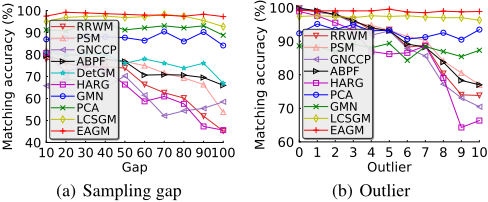
{10, 20, . . . , 100} with 560 image pairs (Figure 3(a)), where increasing gaps indicates deeper deformation; (2) fixing the gap as 50 and evaluating under varying n1 = 30, 29, . . . , 20 (Figure 3(b)), i.e., increasing outliers from 0 to 10. It is obvious that the performance of non-learning methods degrades as the increasing deformation and outliers, but the deep learning methods show relatively stable accuracy. However, only our EAGM is still robust against 100 gaps. On the whole, EAGM outperforms other methods with at least 97.3% accuracy.
These experiments demonstrate that our EAGM with the informative edge semantic features is effective on graph matching with outliers. The fused features also make EAGM more robust, which involves geometric and semantic information jointly.
6 Conclusion
In this paper, we design an edge attention-adaptive graph matching network for graph matching with outliers, named EAGM, to effectively capture the novel edge semantic information that is robust to outliers. EAGM adjusts the impact of each edge on graph matching adaptively, and predicts node and edge binary labels of the associated assignment graph to indicate the matching relations between the two original graphs. Moreover, our novel edge semantic feature not only provides reasonable and independent description for edges, but also distinguishes outliers in the view of their associated edges. The experiments with and without outliers demonstrate that our EAGM achieves promising performance.
Acknowledgments
This work was supported by National Key Research and Development Program of China (No. 2019YFB1406303), National Natural Science Foundation of China (No. 61876003), and Beijing Natural Science Foundation (No. L192024). It is also a research achievement of Key Laboratory of Science, Technology and Standard in Press Industry (Key Laboratory of Intelligent Press Media Technology).
@inproceedings{ijcai2021p134,
  title     = {Adaptive Edge Attention for Graph Matching with Outliers},
  author    = {Qu, Jingwei and Ling, Haibin and Zhang, Chenrui and Lyu, Xiaoqing and Tang, Zhi},
  booktitle = {Proceedings of the Thirtieth International Joint Conference on
               Artificial Intelligence, {IJCAI-21}},
  publisher = {International Joint Conferences on Artificial Intelligence Organization},
  editor    = {Zhi-Hua Zhou},
  pages     = {966--972},
  year      = {2021},
  month     = {8},
  note      = {Main Track},
  doi       = {10.24963/ijcai.2021/134},
  url       = {https://doi.org/10.24963/ijcai.2021/134},
}
TY - CPAPER TI - Adaptive Edge Attention for Graph Matching with Outliers AU - Qu, Jingwei AU - Ling, Haibin AU - Zhang, Chenrui AU - Lyu, Xiaoqing AU - Tang, Zhi T2 - Proceedings of the Thirtieth International Joint Conference on Artificial Intelligence, IJCAI-21 PB - International Joint Conferences on Artificial Intelligence Organization PY - 2021 SP - 966 EP - 972 DO - 10.24963/ijcai.2021/134 UR - https://doi.org/10.24963/ijcai.2021/134 ER -Copied
Machine-readable versions of this paper, for tools and AI agents:





