
Improved CP-Based Lagrangian Relaxation Approach with an Application to the TSP
Proceedings of the Thirtieth International Joint Conference on Artificial Intelligence. Main Track. Pages 1374-1380.
https://doi.org/10.24963/ijcai.2021/190
© 2021 International Joint Conferences on Artificial Intelligence
Keywords
- Constraints and SAT: Constraints: Modeling, Solvers, Applications
- Constraints and SAT: Constraint Optimization
- Constraints and SAT: Global Constraints
Abstract
CP-based Lagrangian relaxation (CP-LR) is an efficient optimization technique that combines cost-based filtering with Lagrangian relaxation in a constraint programming context. The state-of-the-art filtering algorithms for the WeightedCircuit constraint that encodes the traveling salesman problem (TSP) are based on this approach. In this paper, we propose an improved CP-LR approach that locally modifies the Lagrangian multipliers in order to increase the number of filtered values. We also introduce two new algorithms based on the latter to filter WeightedCircuit. The experimental results on TSP instances show that our algorithms allow significant gains on the resolution time and the size of the search space when compared to the state-of-the-art implementation.
- [Applegate et al., 2006] David L. Applegate, Robert E. Bixby, Vasek Chvátal, and William J. Cook. The Travel- ing Salesman Problem: A Computational Study. Princeton University Press, 2006.
- [Bajgiran et al., 2017] Omid Sanei Bajgiran, Andre A. Cire, and Louis-Martin Rousseau. A First Look at Picking Dual Variables for Maximizing Reduced Cost Fixing. In Domenico Salvagnin and Michele Lombardi, editors, Inte- gration of AI and OR Techniques in Constraint Program- ming, Lecture Notes in Computer Science, pages 221-228, Cham, 2017. Springer International Publishing.
- [Beasley, 1993] John E. Beasley. Lagrangian relaxation. In Modern Heuristic Techniques for Combinatorial Prob- lems, pages 243-303.
- [Benchimol et al., 2012] Pascal Benchimol, Willem-Jan van Hoeve, Jean-Charles Régin, Louis-Martin Rousseau, and Michel Rueher. Improved filtering for weighted circuit constraints. Constraints, 17(3):205-233, July 2012.
- [Bergman et al., 2015] David Bergman, Andre A. Cire, and Willem-Jan van Hoeve. Improved Constraint Propaga- tion via Lagrangian Decomposition. In Gilles Pesant, ed- itor, Principles and Practice of Constraint Programming, Lecture Notes in Computer Science, pages 30-38, Cham, 2015. Springer International Publishing.
- [Cambazard and Fages, 2015] Hadrien Cambazard and Jean- Guillaume Fages. New filtering for AtMostNValue and its weighted variant: A Lagrangian approach. Constraints, 20(3):362-380, July 2015.
- [Fages et al., 2016] Jean-Guillaume Fages, Xavier Lorca, and Louis-Martin Rousseau. The salesman and the tree: The importance of search in CP. Constraints, 21(2):145- 162, April 2016.
- [Fages, 2014] Jean-Guillaume Fages. Exploitation de struc- tures de graphe en programmation par contraintes. PhD thesis, Ecole des Mines de Nantes, October 2014.
- [Fahle and Sellmann, 2002] Torsten Fahle and Meinolf Sell- mann. Cost Based Filtering for the Constrained Knapsack Problem. Annals of Operations Research, 115(1):73-93, September 2002.
- [Focacci et al., 1999] Filippo Focacci, Andrea Lodi, and Michela Milano. Cost-Based Domain Filtering. In Joxan Jaffar, editor, Principles and Practice of Constraint Pro- gramming, Lecture Notes in Computer Science, pages 189-203, Berlin, Heidelberg, 1999. Springer.
- [Held and Karp, 1970] Michael Held and Richard M. Karp. The Traveling-Salesman Problem and Minimum Spanning Trees. Operations Research, 18(6):1138-1162, 1970.
- [Held and Karp, 1971] Michael Held and Richard M. Karp. The traveling-salesman problem and minimum spanning trees: Part II. Mathematical Programming, 1(1):6-25, De- cember 1971. [Helsgaun, 2000] Keld Helsgaun. An effective implemen- tation of the Lin-Kernighan traveling salesman heuristic. European Journal of Operational Research, 126(1):106- 130, October 2000.
- [Isoart and Régin, 2019] Nicolas Isoart and Jean-Charles Régin. Integration of Structural Constraints into TSP Mod- els. In Thomas Schiex and Simon de Givry, editors, Prin- ciples and Practice of Constraint Programming, Lecture Notes in Computer Science, pages 284-299. Springer In- ternational Publishing, 2019.
- [Isoart and Régin, 2020] Nicolas Isoart and Jean-Charles Régin. Adaptive CP-Based Lagrangian Relaxation for TSP Solving. In Emmanuel Hebrard and Nysret Musliu, editors, Integration of Constraint Programming, Artificial Intelligence, and Operations Research, Lecture Notes in Computer Science, pages 300-316, Cham, 2020. Springer International Publishing.
- [Jussien et al., 2008] Narendra Jussien, Guillaume Rochart, and Xavier Lorca. Choco: An Open Source Java Con- straint Programming Library. In CPAIOR'08 Workshop on Open-Source Software for Integer and Contraint Program- ming (OSSICP'08), pages 1-10, Paris, France, 2008.
- [Menana and Demassey, 2009] Julien Menana and Sophie Demassey. Sequencing and Counting with the multicost- regular Constraint. In Willem-Jan van Hoeve and John N. Hooker, editors, Integration of AI and OR Techniques in Constraint Programming for Combinatorial Optimization Problems, Lecture Notes in Computer Science, pages 178- 192, Berlin, Heidelberg, 2009. Springer.
- [Reinelt, 1991] Gerhard Reinelt. TSPLIB-A Traveling Salesman Problem Library. ORSA Journal on Computing, 3(4):376-384, November 1991.
- [Sellmann and Fahle, 2001] Meinolf Sellmann and Torsten Fahle. CP-based Lagrangian Relaxation for a Multimedia Application. In 3rd International Workshop on Integration of AI and OR Techniques in Constraint Programming for Combinatorial Optimization Problems (CP-AI-OR), pages 1-14, 2001.
- [Sellmann and Fahle, 2003] Meinolf Sellmann and Torsten Fahle. Constraint Programming Based Lagrangian Relax- ation for the Automatic Recording Problem. Annals of Op- erations Research, 118(1):17-33, February 2003.
- [Sellmann, 2004] Meinolf Sellmann. Theoretical Founda- tions of CP-Based Lagrangian Relaxation. In Mark Wal- lace, editor, Principles and Practice of Constraint Pro- gramming -CP 2004, Lecture Notes in Computer Science, pages 634-647, Berlin, Heidelberg, 2004. Springer.
- [Wolsey, 2020] Laurence Wolsey. Branch and Bound. In In- teger Programming, chapter 7, pages 113-138.
References were extracted automatically from the PDF and may contain errors.
Full text extracted automatically from the PDF; figures, tables and equations may differ. The PDF is the version of record.
1 Introduction
In constraint programming (CP), an efficient way to perform domain filtering for an optimization problem is costbased filtering [Focacci et al., 1999]. Given a minimization problem and an upper bound on the objective value, the cost of a relaxed subproblem is used as lower bound. If assigning a variable to a value increases this lower bound beyond the upper bound, this assignment is inconsistent and the value is filtered out from the variable domain. In linear programming, Lagrangian relaxation is a common technique to obtain lower bounds. Difficult constraints are moved into the objective function while adding weights, called Lagrangian multipliers, that penalize the objective when these constraints are violated. Maximizing the objective function over the multipliers provides better lower bounds. During this optimization process, one could apply cost-based filtering to each of the resulting subproblems. From this idea, CP-based Lagrangian relaxation (CP-LR) was introduced [Sellmann and Fahle, 2001] and used to solve many problems [Fahle and Sellmann, 2002; Sellmann and Fahle, 2003; Menana and Demassey, 2009; Bergman et al., 2015; Cambazard and Fages, 2015]. In particular, the state-ofthe-art filtering algorithms for the WEIGHTEDCIRCUIT constraint that encodes the traveling salesman problem (TSP) are based on a CP-LR approach [Benchimol et al., 2012].
We propose an improved CP-LR approach that adds a step before applying the cost-based filtering. This step globally increases the number of filtered values by locally modifying the Lagrangian multipliers. It results in a stronger filtering and a greater pruning of the search tree.
Section 2 presents the theory of cost-based filtering, Lagrangian relaxation, CP-LR, the TSP, and the WEIGHTEDCIRCUIT constraint. Section 3 describes our improved CP-LR approach. Section 4 presents two new algorithms based on this approach to filter the WEIGHTEDCIRCUIT constraint. Experiments on the TSP (Section 5) show a significant gain on both the resolution time and the size of the search space when compared to the state-of-the-art implementation of WEIGHTEDCIRCUIT [Jussien et al., 2008; Fages, 2014].
2 Background
2.1 Cost-Based Filtering
Consider the generic optimization problem min f(x), where x = (x1, . . . , xn) subject to unspecified constraints. CP generally uses a branch-and-bound approach to explore, within a search tree, the possible assignments for x. Say, at some point of the search, the best solution found has an objective value U and that we can compute a lower bound L by considering a relaxed version of the original problem. Cost-based filtering [Focacci et al., 1999] consists in using the information of the current relaxed subproblem to filter values from the variable domains. If L > U, infeasibility is raised. Let L[xi = µ] be the optimal objective value of the relaxed subproblem with the extra constraint xi = µ. If L[xi = µ] > U, then the value µ is filtered out from dom(xi). This method requires an efficient algorithm to compute L[xi = µ]. In the context of integer linear programming, reduced costs can be used to filter specific values with a similar reasoning (reduced cost fixing, see e.g. [Wolsey, 2020]).
2.2 Lagrangian Relaxation
Consider the following linear program formed of two constraint families, A : Ax ≤ b and B : Bx ≤ d, where X ⊆ Rn is an arbitrary set:
Suppose A consists of difficult constraints. The Lagrangian relaxation technique lets these constraints go in the objective function while keeping a global view on the original problem. Introducing Lagrangian multipliers λi ≥ 0, the objective function is penalized when the constraints of A are violated, resulting in the following relaxed problem:
Any λ ≥ 0 makes ZLR(λ) a valid lower bound of Z. In order to get the tightest bound, the Lagrangian multiplier problem is to find λ that maximizes ZLR(λ) subject to λ ≥ 0. Various methods exist in the literature to solve this problem including subgradient descent algorithms [Beasley, 1993; Sellmann, 2004], where the choice of multipliers is guided by the solution of (LR(λ)) until convergence.
2.3 CP-Based Lagrangian Relaxation
Assume we are given the linear program (P) and that an efficient filtering algorithm PROP(B) is known for B. CP-based Lagrangian relaxation (CP-LR) [Sellmann and Fahle, 2001; Sellmann, 2004] consists of optimizing the Lagrangian multipliers for A while using PROP(B) for each subproblem (LR(λ)) encountered during the gradient descent. Hence, while maximizing the lower bound ZLR(λ) over λ, costbased filtering is applied on the corresponding substructure B.
As shown by Sellmann [2004], suboptimal multipliers can be more efficient for filtering than the multipliers that optimize the bound. This justifies why the filtering should be performed during the multipliers optimization process rather than once at the end. While optimizing the bound is the main objective, one could also want to maximize the quantity of filtered values each time PROP(B) is called. Thus, it is a hint that multipliers should play a greater role in the filtering step.
2.4 TSP and WEIGHTEDCIRCUIT
Let G = (V,E) be an undirected graph with nodes set V := {1, . . . n}, edges set E ⊆ {{x, y} : x, y ∈ V, x ̸= y} and weight function w : E → Z. For an edge {i, j} ∈ E, we write w(i, j) for its weight. The (symmetric) traveling salesman problem (TSP) consists in finding a Hamiltonian cycle in G of minimum weight, i.e. a minimal path visiting all nodes and returning to its starting point.
Let δ(i) := {e ∈ E : i ∈ e} be the set of edges adjacent to node i. Introducing binary variables xe for e ∈ E, the TSP can be modeled as an integer linear program [Applegate et al., 2006]:
Equations (1) are known as the degree constraints and require that each node have exactly two adjacent edges. Inequalities (2) are known as the subtour elimination constraints and ensure the connectivity of the tour.
The 1-tree relaxation of Held and Karp [1970; 1971] results from relaxing the degree constraints (1). Let G′ = (V ′ , E′ ) be the graph G from which an arbitrary node labeled 1 is removed, i.e. with V ′ := V \ {1} and E′ := E \ δ(1). A 1-tree of G is a spanning tree of G′ to which we add two distinct edges adjacent to node 1. The 1-tree relaxation consists in finding a 1-tree of G of minimal weight. The sum of the edges' weights in the 1-tree is a lower bound of the TSP. Introducing Lagrangian multipliers λ = (λ1, . . . , λn) ∈ Rn with λ1 = 0, this lower bound can be improved with a Lagrangian relaxation of the degree constraints (1). Let degA(i) := |{e ∈ A : i ∈ e}| be the degree of node i ∈ V in a set of edges A. We obtain the following relaxed problem:
Observe that the objective function can be rewritten as
Thus, ZLR(λ) can be found by computing a minimum spanning tree of G′ , denoted S, and adding the two minimal edges adjacent to node 1, denoted m1 and m2, using the weight function ˜w(i, j) := w(i, j) + λi + λj , ∀{i, j} ∈ E.
In CP, given the binary variables x = (xe1 , . . . , xe|E| ), the weight function w, and an integer variable z, the WEIGHTEDCIRCUIT(x,w, z) constraint [Benchimol et al., 2012] is satisfied if the edges e ∈ E with xe = 1 form a Hamiltonian cycle on the nodes V with total weight at most z. The TSP is thus formulated as a minimization problem on z subject to this constraint. Its filtering algorithms rely on the identification of mandatory edges that must be part of any solution and forbidden edges that cannot be part of any solution, through the costs stemming from the 1-tree structure.
Let M be the set of mandatory edges and suppose that forbidden edges were removed from E. Let λ be the Lagrangian multipliers, T := S ∪ {m1, m2} the minimum 1-tree and U a known upper bound on the value of Z.
For an edge e ∈ E \ T, the support edge s ∈ T is the edge that needs to be removed from T if e is forced into the minimum 1-tree. If e is not adjacent to node 1, let Ce ⊆ S be the edges lying on the unique cycle in S ∪ {e}. The non-mandatory edge s ∈ Ce \ M with maximum weight is the support edge of e. Else, e is adjacent to node 1 and the support edge s is the one in {m1,m2} \M with the greatest weight. The reduced cost of e, denoted ¯ c(e), is the increase of the objective value when forcing e in T. Thus, we have ¯ c(e) = ˜w(e) - ˜w(s) or ∞ if s does not exist. Cost-based filtering implies that e ∈ E \ T is forbidden if ZLR(λ)[xe = 1] = ZLR(λ) + ¯ c(e) > U.
For an edge e ∈ T , the replacement edge r is the edge that replaces e in the minimum 1-tree if e is removed. If e is not adjacent to node 1, removing e from S divides the tree into two components. We define Re ⊆ E′ \ S to be the cut-set of G′ induced by the removal of edge e fromS, i.e. the edges in E′ adjacent to both components in S \ {e}. The replacement edge r is the one with minimum weight in Re. Otherwise, e is adjacent to node 1 and the replacement edge is the one in
δ(1) \ {m1,m2} with the smallest weight. The replacement cost of e, denoted ˆ c(e), is the increase of the objective value when removing e from T . Thus, we have ˆ c(e) = ˜w(r)- ˜w(e) or ∞ if r does not exist. Cost-based filtering implies that e ∈ T is mandatory if ZLR(λ)[xe = 0] = ZLR(λ) + ˆ c(e) > U.
3 Improved CP-LRApproach
Consider the original problem (P) and its relaxation (LR(λ)). During the optimization of the Lagrangian multipliers λ for A, we look closer at the filtering step of PROP(B) on the subproblem (LR(λ)). We know from Sellmann [2004] that a worse lower bound could lead to more filtering and that this phenomenon is not restricted to CP-LR. Given a variable and a value for which we would like to perform cost-based filtering, could we temporarily change the Lagrangian multipliers so that this value is filtered? In this context, temporarily would mean that we find multipliers to filter the value, but we do not consider them in the general multiplier optimization process. We propose the following general framework:
- Find conditions on the multipliers so that the relaxed solution x∗ = (x∗1 . . . x∗n ) of (LR(λ)) remains optimal.
- For each variable xi and value µ ∈ dom(xi) \ {x∗i }, check whether there exist new multipliers λ′ satisfying the conditions from step 1 such that ZLR(λ′ )[xi = µ] > U. If so, filter µ from dom(xi).
The algorithms executing these steps are left unspecified since the framework depends greatly on the nature of the problem. For any propagator, this approach provides a natural extension: the original cost-based filtering algorithm corresponds to the case where we have λ′ = λ in step 2. Also, note that it can be seen as a generalization of the dual picking technique [Bajgiran et al., 2017].
Consider this integer program with the constraint 3x2 - x3 ≤ 2 relaxed into the objective using a Lagrangian λ ≥ 0:
Suppose we know an efficient cost-based filtering algorithm for this relaxed problem and that an upper bound on Z is -1. Choosing λ = 0, we obtain ZLR(0) = -3, with the solution x∗ = (1, 0, 1). We compute ZLR(0)[x1 = 0] = -2, ZLR(0)[x2 = 1] = -2 and ZLR(0)[x3 = 0] = -1 and no value is filtered from these costs, even if the bound -3 is optimal. With our improved approach, say we want to look more closely to x3 = 0. Step 1, we note that the solution x∗ is optimal for every multiplier λ ≥ 0. Step 2, looking at the subproblem ZLR(λ′ )[x3 = 0], we find that λ′ = 13 leads to ZLR( 1 3 )[x3 = 0] = - 23 > -1. We infer that x3 ̸= 0.
4 Application to the TSP
Given Lagrangian multipliers λ, the state-of-the-art filtering algorithms for the WEIGHTEDCIRCUIT constraint compute a minimum 1-tree and the support/replacement edges of every edge in the graph. A brute-force algorithm directly derived from the definitions computes the reduced/replacement costs as well as the sets Ce or Re for each edge e ∈ E in overall time O(|V ||E|). We propose to apply the improved framework of Section 3 supposing this pre-processing step was done.
Let the relaxed solution x∗ correspond to the minimum 1tree T which gives the lower bound ZLR(λ). By definition of the 1-tree relaxation, this solution is optimal if, and only if, T is a minimum 1-tree of G. Thus, for each edge e ∈ E \M, the search for Lagrangian multipliers λ′ is subject to the condition that T remains a minimum 1-tree of G.
Given an edge {i, j} ∈ E \ M, Lemma 1 specifies the conditions on how to find λ′ that increases the value of ZLR(λ)[x{i,j} = 0] or ZLR(λ)[x{i,j} = 1].
Lemma 1. Let {i, j} ∈ E \ M be an edge of G. Suppose {k, l} is the support (resp. replacement) edge of {i, j} and λ′ := (λ1, . . . , λs+v, . . . , λn) where v ∈ Rand s ∈ V \{1}. If v is chosen such as under this modification T remains a minimum 1-tree of G and {k, l} the support (resp. replacement) edge of {i, j}, then
where 1A(x) = 1 iff x ∈ A is the indicator function.
Proof. Suppose that {i, j} ∈ E \ T and that {k, l} is its support edge (the proof is similar for {i, j} ∈ T). Considering λ′ , let ˜w′ (e) be the new weight of edge e. Since T is still a minimum 1-tree of G and {k, l} the support edge of {i, j}, ZLR(λ′ )[x{i,j} = 1] = ZLR(λ′ ) + ˜w′ (i, j) - ˜w′ (k, l) by definition of the reduced cost of {i, j}. We have
where c = 1{i,j}(s) - 1{k,l}(s) ∈ {-1, 0, 1}. Recalling that
and putting it all together, the result follows.
Even though Lemma 1 imposes the condition that the support/replacement edge of {i, j} remains unchanged, which is more than what is required by the step 1, it leads in the following to a SIMPLE algorithm (Section 4.1) and an α-SETS algorithm (Section 4.2).
4.1 The SIMPLE Algorithm
Given the edge {i, j} ∈ E \ M, the SIMPLE algorithm (Algorithm 1) checks whether λi and λj can be both modified so that dom(x{i,j}) is filtered. If {i, j} ∈ T, line 1 computes the value ∆ corresponding to how much the bound and the replacement cost of {i, j} needs to be increased in order to declare the edge mandatory. For λi, line 2 calls MAXDECREASE to compute a value v ≤ 0 such that λi + v is a modification allowed by the hypotheses of Lemma 1 and that can only increase ZLR(λ)[x{i,j} = 0]. Line 3 performs the same process for λj . If SIMPLE is applied for {i, j} ∈ E \ T , we aim at increasing the values of the multipliers λi and λj so that {i, j} is identified as forbidden. Line 4 computes the value ∆ of how much the bound and the reduced cost of {i, j} need to be increased. For λi, line 5 calls MAXINCREASE to compute a value v ≥ 0 such that λi + v is a modification allowed by the hypotheses of Lemma 1 and that increases ZLR(λ)[x{i,j} = 1]. Line 6 repeats the process for λj .
For {i, j} ∈ T and the multiplier λi, line D1 of function MAXDECREASE computes a value α ≥ 0 ensuring T remains a minimum 1-tree under the modification λi - α. Line D2 restricts this value not to exceed β to ensure that the replacement edge of {i, j} remains unchanged. For {i, j} ∈ E \ T, the value α computed on line I1 of function MAXINCREASE ensures that T remains a minimum 1-tree while the value β computed on line I2 restricts the support edge of {i, j} to remain unchanged. Both functions run in O(|V |).
In the following, we show that for an edge {i, j} ∈ T , the SIMPLE algorithm correctly computes new values for λi and λj that can only increase ZLR(λ)[x{i,j} = 0]. The proof is similar in the case of an edge {i, j} ∈ E \ T. For the modification of λi, we first need the following lemma.
Lemma 2. Considering λ′ = (λ1, . . . , λi - α, . . . , λn) and the corresponding new reduced costs ¯ c′ (e) for e ∈ E \ T , we have ¯ c′ (e) ≥ 0 ∀e ∈ E \ T .
Proof. Consider e ∈ E \ T and let s, s′ ∈ T be respectively the support edge of e before and after considering the multipliers λ′ . We have
because ˜w′ (x) ≤ ˜w(x) ∀x ∈ E and by definition of a support edge, ˜w(s′ ) ≤ ˜w(s). Now, if e ∈ δ(i), we have
by definition of α in line D1. Else, e /∈ δ(i) and
In every case, ¯
By Lemma 2, the reduced costs remain positive, thus T remains a minimum 1-tree under the modification of λi. For every edge a adjacent to i in R{i,j}, a is a candidate to be a replacement edge of {i, j}. If r is the current replacement edge of {i, j}, the value computed by β guarantees that ˜w′ (a) ≥ ˜w′ (r) with the multipliers λ′ , i.e. that r remains the replacement edge. Since v ≤ 0 and the conditions i /∈ {1, k, l}∧degT (i) ≤ 2 hold, the conclusion follows from
Algorithm 1: SIMPLE(i, j)
if {i, j} ∈ T then {k, l} ← GETREPLACEMENTEDGE(i, j) 1 ∆←U - (ZLR(λ) + ˜w(k, l) - ˜w(i, j)) if i /∈ {1, k, l} ∧ degT (i) ≤ 2 then // Decrease λi 2 v ← (-1)·MAXDECREASE(i, j) ∆ ← ∆ - (v · (degT (i) - 2) - v) if j /∈ {1, k, l} ∧ degT (j) ≤ 2 then // Decrease λj 3 v ← (-1)·MAXDECREASE(j, i) ∆ ← ∆ - (v · (degT (j) - 2) - v) if ∆ < 0 then dom(x{i,j}) ← dom(x{i,j}) \ {0} else{k, l} ← GETSUPPORTEDGE(i, j) 4 ∆←U - (ZLR(λ) + ˜w(i, j) - ˜w(k, l)) if i /∈ {1, k, l} ∧ degT (i) ≥ 2 then // Increase λi 5 v ← MAXINCREASE(i, j) ∆ ← ∆ - (v · (degT (i) - 2) + v) if j /∈ {1, k, l} ∧ degT (j) ≥ 2 then // Increase λj 6 v ← MAXINCREASE(j, i) ∆ ← ∆ - (v · (degT (j) - 2) + v) if ∆ < 0 then dom(x{i,j}) ← dom(x{i,j}) \ {1}Function MAXDECREASE(i, j)
D1 α←min{GETREDUCEDCOST(i, k) : {i, k} ∈ E \ T } ∪ {∞} if j ̸= 1 then r ← GETREPLACEMENTEDGE(i, j) D2 β ←min{ ˜w(i, k) - ˜w(r): {i, k} ∈ R{i,j}} ∪ {∞} α ← min{α, β} return αFunction MAXINCREASE(i, j)
I1 α←min{GETREPLACEMENTCOST(i, k) : {i, k} ∈ T \ M} ∪ {∞} if j ̸= 1 then s ← GETSUPPORTEDGE(i, j) I2 β ←min{ ˜w(s)- ˜w(i, k): {i, k} ∈ C{i,j}\M}∪{∞} α ← min{α, β} return αLemma 1. The same process is performed with λj without recomputing the reduced costs. Indeed, the modification of λi cannot decrease the reduced cost of edges adjacent to node j.
SIMPLE only considers specific cases of Lemma 1 and some opportunities of increasing ZLR(λ)[x{i,j} = µ] are ignored. This allows us to assure the previous properties are true and keep the algorithm simple and efficient.
The values computed on lines D2 and I2 require the sets Ce and Re. As an alternative that only uses the reduced costs computed by a faster pre-processing [Benchimol et al., 2012], we propose to replace the sets on lines D2 and I2 by
In the following, we refer to the choice of the original sets as the complete policy and of these latter as the relaxed policy. In both cases, the overall time complexity is in O(|V |).
4.2 The α-SETS Algorithm
Following step 1, we derive the conditions on the multipliers in order for the 1-tree T = S ∪ {m1, m2} to remain minimal.
The constraints (A) come from the cut property of minimum spanning trees stating that the cost of an edge in the tree {a, b} should not be greater than the cost of any edge {c, d} in its cut-set R{a,b}. The constraints (B) ensure that m1 and m2 are the two minimal edges adjacent to node 1. For an edge {i, j} ∈ E \ M, Lemma 1 also requires that its support/replacement edge {k, l} ∈ E \ M remains unchanged. By definition, this can be formulated as
All of these constraints are linear and could be used to derive a linear program that maximizes ZLR(λ′ )[x{i,j} = µ]. However, given there are O(|V |4 ) constraints, even the best linear solvers take too much time for the filtering to pay off. Therefore, we solve an easier problem where constraints are gradually added and multipliers are locally modified.
Given an edge {i, j} ∈ E \ M and Lagrangian multipliers λ, the α-SETS algorithm tries to find an α-set A ⊆ V in the graph: a set of nodes that will have their corresponding multiplier simultaneously modified and that will lead to an increased ZLR(λ)[x{i,j} = µ] value. Each node u ∈ V is labeled with a value σu ∈ {-1, 0, +1} initially set to 0, corresponding to whether the multiplier λu will decrease (-1), increase (+1), remain unchanged (0). For a variable α ≥ 0 and each node u, we look for multipliers λ′u = λu +σu · α. Starting from an initial node, the algorithm computes incrementally a set A of nodes and a set Ω of constraints taken from (A) to (F). During any step in the process, the substitution of λ′u by λu + σu · α ∀u ∈ V in each constraint ω ∈ Ω leads to a system of linear inequalities that can be written in the form cω · α ≤ mω, where the coefficient cω ∈ {-2,-1, 0, 1, 2} and mω ≥ 0 are two known constants. Maximizing α under these constraints, a value α∗ ≥ 0 is found. If α∗ = 0, the algorithm looks for the restraining constraint and appends one of its related nodes to A in order to loosen the inequality. Doing so, new constraints must be taken into account and added to Ω. This process is repeated until α∗ > 0, leading to a valid α-set A and new multipliers λ′ . The increased value ZLR(λ′ )[x{i,j} = µ] directly follows from the sum of all the changes according to Lemma 1, without having to recompute a minimum 1-tree. If it is still insufficient to filter dom(x{i,j}), the procedure can be re-executed with the multipliers λ := λ′ previously found and looks for another α-set.
This procedure searches for an α-set A where {k, l} ∈ E \ M is the support/replacement edge of {i, j}.
- Initialize a set of constraints Ωwith the constraints from (C) to (F), depending on the nature of {i, j}.
- Choose an initial node u ∈ {i, j, k, l} \ {1} and σu ∈ {-1, +1}. Following Lemma 1, this choice must satisfy
(b) {i, j} ∈ T ⇒
σu · (degT (u) - 2 + 1{k,l}(u) - 1{i,j}(u)) > 0.
If none of these 8 combinations works, no set A exists and the algorithm halts without filtering dom(x{i,j}).
- Append node u to the set A.
- Add to Ω all the constraints not already considered of type (A)-(B) where λ′u has coefficient σu.
- For each constraint ω ∈ Ω, compute the values cω and mω. Since ω is of the form λ′c +λ′d -λ′a -λ′b ≤ w(a, b)- w(c, d), we have cω = σa + σb - σc - σd and mω = ˜w(a, b) - ˜w(c, d). The maximal value α ≥ 0 can take, subject to the constraints in Ω, is given by
- If α∗ > 0, return the value α∗ and the set A is found.
- If α∗ = 0, find the constraint ¯ω ∈ Ω that prevents obtaining a value α > 0. This constraint is of the form c¯ω · α ≤ ˜w(a, b) - ˜w(c, d), where a, b, c, d ∈ V .
- Choose a node u′ ∈ {a, b, c, d} \ {1} and σu′ ∈ {-1, +1} such that
- (a) u′ /∈ P ∪ ({a, b} ∩ {c, d});
- (b) (u′ ∈ {a, b} ∧ degT (u′ ) ≥ 2) ⇒ σu′ = +1;
- (c) (u′ ∈ {c, d} ∧ degT (u′ ) ≤ 2) ⇒ σu′ = -1;
- (d) u′ ∈ {i, j, k, l} ⇒ conditions of step 2.
If none of these 8 combinations works, backtrack and reconsider the last choice. If no possibility remains, no set A exists and the algorithm halts without filtering dom(x{i,j}). Else, set u := u′ and go to step 3.
Since the procedure can be repeated as long as an α-set A is found and dom(x{i,j}) is not filtered, a maximum number of iterations can be added. Also, to avoid considering too many constraints at the same time, a maximum cardinality Cm on A can be imposed. Our implementation follows an iterativedeepening search that gradually increases Cm. For an α-set of C nodes, step 5 deals with C · O(|V ||E|) constraints. As 4 nodes are possible for each choice, it leads to a worst-case time complexity in O(Cm|V ||E|4Cm ).
This algorithm can be combined with the SIMPLE algorithm and the complete policy: we call the latter first to obtain new multipliers λ′ , and if it was not enough to filter the considered edge, we use them as the initial multipliers for αSETS. We refer to this process as the HYBRID algorithm.
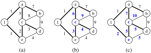
4.3 Example
On the graph of Figure 1a with ZLR(λ) = 19 and U = 23, {a, b} is the support edge of {b, c} and ZLR(λ)[x{b,c} = 1] = ZLR(λ) + ˜w(b, c) - ˜w(a, b) = 20. We apply HYBRID on edge {b, c}. First, SIMPLE finds that λc can be increased by 1, obtained from the minimum between α = 1 (line I1) and β = 2 (line I2). This leads to the multipliers λ′ on Figure 1b, but ZLR(λ′ )[x{b,c} = 1] = 22 ≤ U. Choosing again to increase node c by α ≥ 0, α-SETS finds the constraint α ≤ ˜w′ (d, e) - ˜w′ (c, d) = 0. A valid choice is to simultaneously increase node e by α, leading to the new constraint α ≤ ˜w′ (d, e) - ˜w′ (c, e) = 1. Since α∗ > 0, the multipliers λ′ are updated (Figure 1c) and ZLR(λ′ )[x{b,c} = 1] = 24 > U. The edge {b, c} is thus forbidden.
5 Experiments
The algorithms were implemented 1 in Java 14 using the solver Choco 4.0.6 [Jussien et al., 2008] and its extension Choco Graph 4.2.3 [Fages, 2014]. The experiments were performed on a CentOS Linux 7 machine using an Intel Xeon Silver 4110 CPU at 2.10 GHz and 32 GB of RAM. The TSP was modeled using the WEIGHTEDCIRCUIT constraint already implemented in Choco Graph using the state-of-the-art algorithms [Benchimol et al., 2012]. It uses a subgradient descent algorithm to optimize the Lagrangian multipliers. We kept the default parameters, but we did not restart the algorithm when the lower bound of the 1-tree was increased. As an initial upper bound on the objective variable, we gave the bound provided by the LKH-2.0.9 heuristic [Helsgaun, 2000]. The search strategy was fixed to maxCost with the LCFirst policy [Fages et al., 2016]. We chose the symmetric TSP instances from the TSPLIB library [Reinelt, 1991] between 96 and 500 nodes that could be solved by Choco under 8 hours and with at least 100 search nodes.
We compare the SIMPLE and HYBRID algorithms against the one from Choco. Our algorithms were only called at the very last iteration of the subgradient process. Furthermore, for HYBRID, since α-SETS is slowed down by the number of constraints, it was only called when |E| ≤ 2|V | with a limit of 2 on the cardinality of the α-sets and a maximum of 10 iterations when trying to reach the fixed point.
1 The code is available at http://www2.ift.ulaval.ca/∼quimper/ publications.php.
| Instance | Choco | SIMPLE Relaxed | SIMPLE Complete | HYBRID | ||||
|---|---|---|---|---|---|---|---|---|
| N | T | N | T | N | T | N | T | |
| gr96 | 520 | 3.2 | 436 | 2.7 | 365 | 2.4 | 323 | 2.4 |
| kroA100 | 1488 | 8.3 | 1066 | 5.9 | 1211 | 6.8 | 873 | 5.5 |
| kroB100 | 2312 | 12.3 | 1838 | 8.9 | 2042 | 11.0 | 1462 | 7.9 |
| kroC100 | 360 | 2.3 | 247 | 1.5 | 263 | 1.7 | 210 | 1.5 |
| kroD100 | 128 | 1.1 | 132 | 1.0 | 127 | 1.0 | 114 | 0.9 |
| kroE100 | 1915 | 9.8 | 1578 | 8.4 | 1532 | 8.8 | 1113 | 6.9 |
| gr120 | 324 | 3.0 | 199 | 1.9 | 254 | 2.5 | 145 | 1.6 |
| pr124 | 224 | 2.5 | 195 | 2.1 | 169 | 2.1 | 157 | 1.9 |
| ch130 | 908 | 8.7 | 768 | 7.5 | 673 | 7.2 | 518 | 5.4 |
| pr136 | 72574 | 561.4 | 78781 | 558.2 | 72224 | 503.0 | 66481 | 519.3 |
| gr137 | 923 | 9.9 | 716 | 8.1 | 756 | 9.4 | 746 | 9.8 |
| pr144 | 149 | 2.8 | 65 | 1.3 | 66 | 1.4 | 62 | 1.4 |
| ch150 | 934 | 10.9 | 681 | 7.8 | 710 | 9.6 | 498 | 7.3 |
| kroA150 | 5652 | 65.0 | 2461 | 26.8 | 2910 | 35.4 | 2329 | 27.4 |
| kroB150 | 112078 | 1218.6 | 109715 | 1115.5 | 85765 | 925.6 | 67134 | 671.2 |
| pr152 | 335 | 6.2 | 641 | 9.4 | 446 | 8.2 | 277 | 5.7 |
| si175 | 38068 | 486.0 | 35755 | 436.1 | 38775 | 520.6 | 29915 | 387.3 |
| rat195 | 18785 | 361.1 | 14905 | 290.3 | 13113 | 266.0 | 10281 | 215.9 |
| d198 | 5702 | 101.4 | 7322 | 112.2 | 6695 | 109.0 | 6765 | 118.1 |
| kroA200 | 1176978 | 15766.3 | 863416 | 12654.3 | 884545 | 12399.6 | 687347 | 9618.6 |
| kroB200 | 46484 | 739.2 | 33405 | 555.6 | 32779 | 514.3 | 27392 | 430.0 |
| gr202 | 1568 | 20.2 | 991 | 11.9 | 853 | 11.8 | 644 | 10.0 |
| tsp225 | 125761 | 2426.2 | 72357 | 1416.6 | 74639 | 1546.7 | 51766 | 1174.0 |
| gr229 | 458131 | 7367.2 | 303679 | 4568.1 | 268029 | 4559.1 | 215354 | 3272.8 |
| pr264 | 123 | 8.8 | 130 | 8.9 | 114 | 10.0 | 88 | 8.6 |
| a280 | 1605 | 30.7 | 2429 | 40.2 | 1832 | 33.7 | 2005 | 37.3 |
| lin318 | 3794 | 115.1 | 2296 | 72.8 | 2409 | 81.7 | 1128 | 39.1 |
| gr431 | 415036 | 20485.0 | 309152 | 17077.4 | 278439 | 15917.5 | 241454 | 15074.7 |
| Mean | 89031 | 1779.8 | 65906 | 1393.3 | 63276 | 1339.5 | 50592 | 1130.8 |
Table 1 shows considerable gains on the solving time and the size of the search space for almost every instance. SIMPLE with the relaxed policy gain an average reduction of 15% on the number of nodes and 18% on the solving time. The solving time is reduced for 86% of the instances. Conclusions are similar for the complete policy. However, the gains between the two policies are in general not significant enough to prefer the latter. The improvement is more prominent with the HYBRID algorithm. On average, the number of nodes and the solving time are respectively reduced by 36% and 30% compared to Choco. The solving time is reduced for 93% of the instances. It is in general the best method among all the ones we tested (79% of the instances). In rare cases (a280, d198), the number of nodes increases despite the potential amount of additional filtering. This pathological situation is a well-known fact in the context of CP-LR [Sellmann, 2004; Isoart and R´egin, 2020] and should be more investigated.
6 Conclusion
We introduced an improved approach for CP-LR problems that adds a new step in the filtering process to increase the number of filtered values. We applied it on the WEIGHTEDCIRCUIT constraint filtering by introducing two new algorithms: SIMPLE and α-SETS. Experimental results on TSP instances show they greatly improve the solving time compared to the state-of-the-art implementation of Choco. The recent work of Isoart and R´egin on the TSP (k-cutset [2019], SSSA [2020]) is a priori completely compatible with our work and should be further investigated. Future research also includes testing the approach in other CP-LR contexts.
@inproceedings{ijcai2021p190,
  title     = {Improved CP-Based Lagrangian Relaxation Approach with an Application to the TSP},
  author    = {Boudreault, Raphaël and Quimper, Claude-Guy},
  booktitle = {Proceedings of the Thirtieth International Joint Conference on
               Artificial Intelligence, {IJCAI-21}},
  publisher = {International Joint Conferences on Artificial Intelligence Organization},
  editor    = {Zhi-Hua Zhou},
  pages     = {1374--1380},
  year      = {2021},
  month     = {8},
  note      = {Main Track},
  doi       = {10.24963/ijcai.2021/190},
  url       = {https://doi.org/10.24963/ijcai.2021/190},
}
TY - CPAPER TI - Improved CP-Based Lagrangian Relaxation Approach with an Application to the TSP AU - Boudreault, Raphaël AU - Quimper, Claude-Guy T2 - Proceedings of the Thirtieth International Joint Conference on Artificial Intelligence, IJCAI-21 PB - International Joint Conferences on Artificial Intelligence Organization PY - 2021 SP - 1374 EP - 1380 DO - 10.24963/ijcai.2021/190 UR - https://doi.org/10.24963/ijcai.2021/190 ER -Copied
Machine-readable versions of this paper, for tools and AI agents:





