
Heuristic Search for Approximating One Matrix in Terms of Another Matrix
Proceedings of the Thirtieth International Joint Conference on Artificial Intelligence. Main Track. Pages 1600-1606.
https://doi.org/10.24963/ijcai.2021/221
Keywords
- Machine Learning: Dimensionality Reduction
- Heuristic Search and Game Playing: Heuristic Search
- Data Mining: Feature Extraction, Selection and Dimensionality Reduction
- Machine Learning: Learning Sparse Models
Abstract
We study the approximation of a target matrix in terms of several selected columns of another matrix, sometimes called "a dictionary".
This approximation problem arises in various domains, such as signal processing, computer vision, and machine learning.
An optimal column selection algorithm for the special case where the target matrix has only one column is known since the 1970's,
but most previously proposed column selection algorithms for the general case are greedy.
We propose the first nontrivial optimal algorithm for the general case, using a heuristic search setting similar to the classical A* algorithm.
We also propose practical sub-optimal algorithms in a setting similar to the classical Weighted A* algorithm.
Experimental results show that our sub-optimal algorithms compare favorably with the current state-of-the-art greedy algorithms.
They also provide bounds on how close their solutions are to the optimal solution.
- [Amaldi and Kann, 1998] E. Amaldi and V. Kann. On the approx- imability of minimizing nonzero variables or unsatisfied relations in linear systems. Theoretical Computer Science, 209, 1998.
- [Arai et al., 2015] H. Arai, C. Maung, and H. Schweitzer. Optimal column subset selection by A-Star search. In AAAI'15, pages 1079-1085, 2015.
- [Arai et al., 2016] H. Arai, C. Maung, K. Xu, and H. Schweitzer. Unsupervised feature selection by heuristic search with provable bounds on suboptimality. In AAAI'16, pages 666-672, 2016.
- [Belmerhnia et al., 2014] Leila Belmerhnia, El-Hadi Djermoune, and David Brie. Greedy methods for simultaneous sparse approx- imation. In 2014 22nd European Signal Processing Conference (EUSIPCO), pages 1851-1855, 2014.
- [Bertsimas et al., 2016] Dimitris Bertsimas, Angela King, and Rahul Mazumder. Best subset selection via a modern optimiza- tion lens. The Annals of Statistics, 44(2):813-852, 2016.
- [Bertsimas et al., 2020] Dimitris Bertsimas, Bart Van Parys, et al. Sparse high-dimensional regression: Exact scalable algorithms and phase transitions. The Annals of Statistics, 48(1), 2020.
- [Boutsidis et al., 2013] C. Boutsidis, P. Drineas, and M. Magdon- Ismail. Near-optimal coresets for least-squares regression. IEEE Transactions on Information Theory, 59(10):6880 -6892, 2013.
- [Bunch et al., 1978] J. R. Bunch, C. P. Nielsen, and D. C. Sorensen. Rank-one modification of the symmetric eigenproblem. Numer. Math., 31:31-48, 1978.
- [Chen and Huo, 2006] J. Chen and X. Huo. Theoretical results of sparse representations of multiple measurement vectors. IEEE Transactions on Signal processing, 54(12):4634-4643, 2006.
- [Chen et al., 1989] Sheng Chen, Stephen A Billings, and Wan Luo. Orthogonal least squares methods and their application to non- linear system identification. International Journal of control, 50(5):1873-1896, 1989.
- [Civril and Magdon-Ismail, 2012] A. Civril and M. Magdon- Ismail. Column subset selection via sparse approximation of SVD. Theoretical Computer Science, 421:1-14, March 2012.
- [Cotter et al., 2005] S. Cotter, B. Rao, K. Engen, and K. Kreutz- Delgado. Sparse solutions to linear inverse problems with multi- ple measurement vectors. ASP, 53(7):2477-2488, 2005.
- [Davis et al., 1997] Geoff Davis, Stephane Mallat, and Marco Avel- laneda. Adaptive greedy approximations. Constructive approxi- mation, 13(1):57-98, 1997.
- [Furnival and Wilson, 1974] G. M. Furnival and R. W. Wilson. Re- gressions by leaps and bounds. Technometrics, 16(4):499-511, 1974.
- [Golub and Van-Loan, 2013] G. H. Golub and C. F. Van-Loan. Ma- trix Computations. Johns Hopkins University Press, Baltimore, fourth edition, 2013.
- [Halko et al., 2011] N. Halko, P. G. Martinsson, and J. A. Tropp. Finding structure with randomness: Probabilistic algorithms for constructing approximate matrix decompositions. SIAM Review, 53(2):217-288, 2011.
- [Hansen and Zhou, 2007] Eric A Hansen and Rong Zhou. Any- time heuristic search. Journal of Artificial Intelligence Research, 28:267-297, 2007.
- [Hart et al., 1968] Peter E Hart, Nils J Nilsson, and Bertram Raphael. A formal basis for the heuristic determination of mini- mum cost paths. IEEE transactions on Systems Science and Cy- bernetics, 4(2):100-107, 1968.
- [Hastie et al., 2009] T. Hastie, R. Tibshirani, and J. Friedman. The Elements of Statistical Learning, section 3.3.1. Springer, 2009.
- [He et al., 2019] B. He, S. Shah, C. Maung, G. Arnold, G. Wan, and H. Schweitzer. Heuristic search algorithm for dimensional- ity reduction optimally combining feature selection and feature extraction. In AAAI'19, pages 2280-2287, California, 2019.
- [Hou et al., 2017] C. Hou, Y. Jiao, F. Nie, T. Luo, and Z. Zhou. 2d feature selection by sparse matrix regression. IEEE Transactions on Image Processing, 26(9):4255-4268, 2017.
- [Huang et al., 2020] S. Huang, Y. Peng, C. Chang, K. Cheng, S. Huang, and B. Chen. Restoration of images with high-density impulsive noise based on sparse approximation and ant-colony optimization. IEEE Access, 8, 2020.
- [Mallat, 1999] S. Mallat. A wavelet Tour of Signal Processing. Aca- demic Press, 1999.
- [Maung and Schweitzer, 2015] C. Maung and H. Schweitzer. Im- proved greedy algorithms for sparse approximation of a matrix in terms of another matrix. IEEE Transactions on Knowledge and Data Engineering, 27(3):769-780, March 2015.
- [Natarajan, 1995] B. K. Natarajan. Sparse approximate solutions to linear systems. SIAM Journal of Computing, 25(2):227-234, 1995.
- [Pearl, 1984] J. Pearl. Heuristics : intelligent search strategies for computer. Addison-Wesley, Reading, Massachusetts, 1984.
- [Pohl, 1970] Ira Pohl. Heuristic search viewed as path finding in a graph. Artificial intelligence, 1(3-4):193-204, 1970.
- [Qian et al., 2015] C. Qian, Y. Yu, and Z. Zhou. Subset selection by pareto optimization. In C. Cortes, N. D. Lawrence, D. D. Lee, M. Sugiyama, and R. Garnett, editors, NIPS'15, pages 1774- 1782.
- Curran Associates, Inc., 2015.
- [Qin et al., 2018] Zhijin Qin, Jiancun Fan, Yuanwei Liu, Yue Gao, and Geoffrey Ye Li. Sparse representation for wireless communi- cations: A compressive sensing approach. IEEE Signal Process- ing Magazine, 35(3):40-58, 2018.
- [Selesnick, 2017] I. Selesnick. Sparse regularization via convex analysis. IEEE Transactions on Signal Processing, 65(17), 2017.
- [Shitov, 2017] Y. Shitov. Column subset selection is np-complete, January 2017. arXiv e-print (arXiv:1701.02764[math.CO]).
- [Tibshirani, 1996] R. Tibshirani. Regression shrinkage and selec- tion via the lasso. J. Royal. Statist. Soc B., 58(1):267-288, 1996.
- [Tropp et al., 2006] J. A. Tropp, A. C. Gilbert, and M. J. Strauss. Algorithms for simultaneous sparse approximation. part I: Greedy pursuit. Signal Processing, 86(3):572-588, 2006.
- [Tropp, 2004] J. A. Tropp. Greed is good: algorithmic results for sparse approximation. IEEE Transactions on Information The- ory, 50(10):2231-2242, 2004.
- [Wan and Schweitzer, 2021a] G. Wan and H. Schweitzer. Accel- erated combinatorial search for outlier detection with provable bound on sub-optimality. In AAAI'21, 2021.
- [Wan and Schweitzer, 2021b] Guihong Wan and Haim Schweitzer. A fast algorithm for simultaneous sparse approximation. In 25th Pacific-Asia Conference on Knowledge Discovery and Data Min- ing (PAKDD'21), pages 42-54. Springer, 2021.
- [Zhang, 2009] T. Zhang. Adaptive forward-backward greedy algo- rithm for sparse learning with linear models. In NIPS'09, pages 1921-1928, 2009.
References were extracted automatically from the PDF and may contain errors.
Full text extracted automatically from the PDF; figures, tables and equations may differ. The PDF is the version of record.
1 Introduction
Let Y = (y1 . . . yN) be a "target" matrix of m rows and N columns. Let X = (x1 . . . xn) be a "dictionary" matrix of m rows and n columns. We consider the problem of selecting k ≤ n columns from X that can be used to linearly approximate Y as follows:
where S = (xs1 . . . xsk ) is the selection matrix of size m×k, and A is the coefficient matrix of size k×N. We evaluate the quality of the selected columns in S with the Frobenius norm:
This formulation includes several well-known special cases. Supervised column subset selection corresponds to the case where N = 1. See, e.g. [Hastie et al., 2009; Boutsidis et al., 2013]. When N > 1, the problem is sometimes known as sparse multi-target prediction, or simultaneous sparse approximation (e.g., [Tropp, 2004; Maung and Schweitzer, 2015; Wan and Schweitzer, 2021b]). When Y = X, it is known as the unsupervised column subset selection, or unsupervised feature selection problem (e.g., [Golub and Van-Loan, 2013; Arai et al., 2015]).
Optimal solutions, as well as approximations within a constant, are known to be NP-hard even for the N = 1 case [Natarajan, 1995; Davis et al., 1997; Amaldi and Kann, 1998], and for the unsupervised case where Y = X [Shitov, 2017]. This implies that optimal solutions cannot be efficient. Previous studies have developed optimal algorithms that are exponential in the worst case but improve on exhaustive search, and fast algorithms that are not optimal.
Optimal algorithms for the unsupervised case (Y = X) were studied in [Arai et al., 2015; He et al., 2019]. Optimal algorithms for the N = 1 case were studied in [Furnival and Wilson, 1974; Bertsimas et al., 2016; Bertsimas et al., 2020]. We are not aware of previous studies of optimal algorithms for the N > 1 case that we focus on in this paper.
The case in which the matrix to be approximated contains only one column (N = 1) has received a lot of attention. See, e.g. [Furnival and Wilson, 1974; Qian et al., 2015; Bertsimas et al., 2016; Hou et al., 2017; Qin et al., 2018; Huang et al., 2020]. Applications include signal processing (e.g., [Selesnick, 2017; Qin et al., 2018]) and supervised feature selection in linear regression (e.g., [Furnival and Wilson, 1974; Qian et al., 2015; Hou et al., 2017; Bertsimas et al., 2016]). Convex relaxation approaches to feature selection replace some natural constraints (sometimes defined in terms of l0 norm) with other convex constraints. An example is that the l1 norm is used in the Lasso technique [Tibshirani, 1996]. Another recent variant is the Pareto technique [Qian et al., 2015], where the authors treated the subset selection as a bi-objective optimization problem. The algorithm was proved to be optimal for data drawn from Exponential Decay distributions.
Heuristic search algorithms were recently applied to the unsupervised case where Y = X. See [Arai et al., 2015; Arai et al., 2016; He et al., 2019]. They model the selection as a graph search problem, and apply the A∗ or Weighted A∗ to solve it. Our method is motivated by this approach. The algorithms developed in these studies can be viewed as special cases of our method.
In the general case, the matrix Y contains N > 1 columns. We observe that one cannot simply apply an algorithm for the N=1 case separately to each column of Y . The challenge of the general case is to find columns in X that can simultaneously approximate all columns of Y . Previously proposed algorithms for this general case are generally greedy. They include [Maung and Schweitzer, 2015; Belmerhnia et al., 2014; Civril and Magdon-Ismail, 2012; Tropp et al., 2006]. Some of these algorithms are generated from the greedy algorithms for the N = 1 case. For example, the Simultaneous Orthogonal Matching Pursuit (SOMP) Algorithm [Tropp et al., 2006] was generated from the Orthogonal Matching Pursuit (OMP) [Tropp, 2004]. Similarly, the Simultaneous Orthogonal Least Squares (SOLS) Algorithm [Cotter et al., 2005] is a direct generalization of the Orthogonal Least Squares (OLS) Algorithm [Chen et al., 1989]. An algorithm established in [Civril and MagdonIsmail, 2012] improves the SOLS in term of runtime at the cost of increased memory. A recursive formulation in [Maung and Schweitzer, 2015] is used to improve the speed of the SOLS. A spectral pursuit algorithm presented in [Wan and Schweitzer, 2021b] is efficient when n and N are large. The running time and the memory requirements of these algorithms are summarized in Table 1. The complexity of our greedy variant is discussed in Section 4.
| Algorithms | Time complexity | Memory complexity |
|---|---|---|
| SOMP [Tropp et al., 2006] | O(kmnN) | O(m(N + k)) |
| SSBR [Belmerhnia et al., 2014] | O(TkmnN) | O(m(N +k)) |
| SOLS [Cotter et al., 2005] | O(kmnN) | O(m(n + N)) |
| CM [Civril and Magdon-Ismail, 2012] | O(nN(m+k)) | O(m(n+N)) +nN |
| ISOLS [Maung and Schweitzer, 2015] | O(mnN) | O(km) + 2n |
| SPXY [Wan and Schweitzer, 2021b] | O(km(n+N)) | O(m(n+N)) |
| Greedy variant (this work) | O((k2 +m)rxn) | O(rxn) |
1.1 Our Approach
We propose a heuristic search approach for solving the general problem of selecting a subset of k columns from the dictionary matrix to simultaneously approximate the entire target matrix. Our heuristic functions are based on eigenvalues of related matrices. With proper selection of the heuristics, our algorithm can be tuned to give an optimal solution as well as approximate solutions. The optimal variant runs slow and works only for small k or small dictionary matrices. The suboptimal variants run much faster and produce solutions with guarantees on how close the solutions are to the optima. The main contributions are summarized below:
- We describe the first nontrivial algorithm guaranteed to produce an optimal solution for the general case N ≥ 1.
- We describe suboptimal algorithms that are more accurate than the greedy variants. Their solutions come with bounds on how far the solutions are from the optimal solution.
- We describe a greedy algorithm that produces results of similar accuracy to the current state of the art with a superior running time. It also comes with a bound on how far the solution is from the optimum.
2 The Proposed Algorithms
Heuristic search algorithms on graphs, such as A∗ [Hart et al., 1968] and Weighted A∗ [Pohl, 1970], are widely used for solving search problems that can be modeled as graph search.
Algorithm 1 The Search Algorithm.
Input:
Y : a target matrix of N columns.
- X: a dictionary matrix of n columns.
- k: the desired number of columns to be selected fromX.
- f(⋅): a heuristic function.
- ry (optional): the desired rank of Y . Default:ry=min(m,N). rx (optional): the desired rank of X. Default:rx=min(m, n). Output: a subset S of k columns.
Data Structures: Two global lists of subsets: the fringe list F, and the closed list C.
Preprocessing: Dimensionality reduction.
Initialization: Put the empty subset into F.
- 1: while F is nonempty do
- 2: Pick node ni (associatedwith subset Si of size ki) with the smallest heuristic fi from F. Ties are resolved in favor of the larger ki.
- 3: if Si contains k columns then
- 4: Stop and return Si as the solution subset.
5: else 6: for each child nj of ni do 7: if nj is not in C then 8: Compute fj for nj. 9: Put nj in C. 10: Put nj in F. 11: end if 12: end for 13: end if 14: end whileThe goal is to find a path from a root node to a goal node minimizing the cost associated with the path. The search is guided by functions associated with each node that are known as "Heuristics". With some heuristics, A∗ is guaranteed to be optimal, but it may be very slow. Experimental results and theoretical analysis (e.g., [Pearl, 1984]) show that Weighted A∗ runs faster than A∗ . The algorithm we propose in this paper is similar to the standard (Weighted) A∗ .
We describe the search algorithm in terms of a general heuristic function that will be defined later. It is shown in Algorithm 1. The same search procedure (with different heuristics) was also used in [Arai et al., 2015; Arai et al., 2016; He et al., 2019; Wan and Schweitzer, 2021a].
In our case, the graph is constructed as follows. A node contains a subset of selected columns from X and the corresponding f value based on the approximation error of Y . The root node corresponds to the empty subset. A goal node corresponds to a subset of k columns. The children of a node are created by adding a new column into its parent subset. Without loss of generality, we do not distinguish between a node and a subset. The goal of the algorithm is to search a node of k columns on the graph, minimizing the heuristic function f . The fringe list F is a list of nodes that need to be further evaluated, and the closed list C is a list of visited nodes that need not to be added into F again. Employing the standard "best first" strategy the algorithm selects the node from F with the smallest f value to be expanded.
There are two differences between the search procedure in Algorithm 1 and the typical (Weighted) A∗ procedure. The first is in Line 9, where the node is immediately inserted into the closed list, and the second is in Line 10, where the classical A∗ algorithm first checks if the node is already in the fringe list, and if so decides whether its value needs to be updated. The justification for these differences is that in our case all paths leading from the root node to a node are equivalent. Once a subset node is added into the fringe list other nodes with the same subset (obtained through a different path) will have the exact same heuristic values and therefore can be ignored. This implies that the fringe list is a subset of the closed list. (These observations show that the closed list can be implemented by a hash table, and the fringe list by a heap.)
3 Heuristic Functions
Recall that the error of approximating Y by a linear combination of k columns in S is given by (2). Let ni be an arbitrary subset node. Let ki<k be the number of columns selected at ni, and let Si be the matrix formed by these columns. Let ki=k-ki be the number of columns that still need to be selected. We consider the error that can be obtained by completing Si to size k. Let Si of size ki be such completion. Its error is given by:
In the equation above, E() is the error defined in (2), and Ai,Ai are arbitrary coefficient matrices. Thus, the smallest error of a solution subset that contains Si would be:
This shows that the best choice for the heuristic value fi for a node ni is fi = di. Unfortunately, computing di is too expensive since it requires going over all the subsets Si of size ki. However, we show that there is an effective computational approach to approximate di. We define two approximations li and ui, and show that they bound di from below and above.
where A∗i = argminAi ∥Y - SiAi∥2F , Yi = Y -SiA∗i , Y i is the best rank ki approximation to Yi.
Lemma 1. For any selection Si of size ki ≤ k:
with equality if ki = k.
Proof:
- To prove the right hand side inequality, observe that for any Si the expression for ui is the same as di if the matrix Ai is taken to be identically 0. This ignores the contribution of additional columns that may reduce the error further.
- To prove the left hand side inequality:
The justification for the inequality in (note1) is that the rank of SiAi is at most ki.
- It remains to show that the inequalities become equalities when ki = k. Under this condition, we have: ki = 0, which implies that Y i = 0 and Si = 0. Therefore, li, di and ui have same expression: ∥Yi∥2F . ∎
3.1 Three Variants of the Search Algorithm
Clearly, the best choice for the heuristic function is fi = di. However since it cannot be efficiently calculated, we consider the linear combination between li and ui. Three options of the heuristic function are considered. The resulting variants are stated as in the following theorems.
Theorem 1. (the optimal variant) If fi = li then the algorithm is guaranteed to terminate with an optimal solution.
Theorem 2. (the greedy variant) If fi = ui then the algorithm is greedy and terminates after expanding k nodes.
Theorem 3. (the weighted variant) If fi = li+γui, where γ≥0, and the algorithm terminates with the subset S∗∗ that has an error of e∗∗ then
where e∗ is the smallest possible error.
3.2 Lemmas
Our proofs of the theorems require the following results.
Lemma 2. If nj is a child of ni then li ≤ lj.
Lemma 3. If nj is a child of ni then uj ≤ ui.
Lemma 4. Consider the choice fi = ui. Let ni be the node picked at Line 2 of the algorithm. Then the following two properties hold:
- For each child nj of ni, the selection size ∣Sj ∣ is larger than the selection size of all nodes currently in the fringe list. b. The next node to be picked up will be a child of ni.
Instead of proving Theorem 3 directly, we prove a stronger version with a tighter bound:
Theorem 4. (the tighter weighted variant) If fi = li+γui, where γ≥0, and the algorithm terminates at the node n∗∗ with the subset S∗∗ that has an error of e∗∗ , then:
where e∗ is the smallest possible error, l∗∗ is the value of the lower bound for n∗∗, and umax be the largest value of the upper bound for the nodes remaining in the fringe after the goal node is reached.
To see that Theorem 4 implies Theorem 3, observe that umax ≤ ∥Y ∥2F and l∗∗ ≥ 0.
Lemma 5. Suppose Theorem 4 is false. Then for any node nz on the path from the root to an optimal goal node n∗, the following condition holds: fz < f∗∗.
Similar theorems were proved in [He et al., 2019] for the unsupervised case. However, the proof technique used in their study does not appear strong enough to prove these theorems for the supervised case. The tool we use to prove the lemmas is the interlacing property of eigenvalues [Golub and Van-Loan, 2013].
The proof of Theorem 1 follows as a corollary of Theorem 3 with γ = 0. Using Lemma 4, Theorem 2 can be proved. Theorem 3 follows from Theorem 4, and Theorem 4 can be proved by contradiction and using the results in Lemma 5. Detailed proofs are given in a supplementary material.
4 Efficient Heuristics Calculation
The following theorem summarizes the computational formulas for heuristic values.
Theorem 5. At the node ni where the ki columns in Si have already been selected from X, additional ki=k-ki columns still need to be selected. Define: Bi = YiY T i , where Yi is defined in (5). Let λ1, . . . ,λm be the eigenvalues of Bi in non-increasing order. Then the values of li,ui defined in (5) can be calculated by:
The proof is given in a supplementary material. From the formulas in Theorem 5, it is clear that only the top ki eigenvalues of Bi need to be calculated in addition to its trace. But they have to be calculated for each node, which is impractical. We proceed to show that there is a matrix related to Bi with a special structure that enables efficient computation of these eigenvalues.
Observe that we only need heuristics for the children of the picked node (parent) at Line 8 in the algorithm. At that point the parent node ni is known. We show how to efficiently calculate the heuristics for the children by first performing an expensive eigendecomposition of the parent. However the expensive eigendecomposition of the parent can be reduced by computing eigendecomposition in the initial preprocessing step. In summary, we discuss three different types of eigendecompositions. The first one is the one in the preprocessing step, which only needs to be performed once. The second is for each parent, and the third is for the children, where only the eigenvalues are needed.
4.1 Initial Eigendecomposition
In the preprocessing step we compute the eigenvalues and the eigenvectors of the matrices By = Y Y T and Bx = XXT . The eigenvalue decompositions give:
where Uy,Ux are the eigenvectors and Dy,Dx are diagonal matrices with the eigenvalues as the diagonal elements.
Let ry be the rank of Y then ry ≤ min(m,N). Let rx be the rank of X then rx ≤ min(m, n). As we show later we can ignore zero eigenvalues and their corresponding eigenvectors, and can replace X, Y with the following information:
With the advancement of randomized algorithms for matrix decompositions, this initial step can be performed efficiently. For example, using the algorithm described in [Halko et al., 2011], the time complexity is O(mryN+mrxn); the memory complexity is O(mry+mrx+rxn) for the preprocessing step.
4.2 Eigendecomposition for Parent Nodes
Instead of working with the matrix Bi as defined in Theorem 5, we use a related matrix Hi which has same eigenvalues as Bi. The special structure of Hi makes the calculations of these eigenvalues more efficient.
Lemma 6. Let Qi be an orthonormal basis of the current selection Si (selected fromX) of size ki. Let ˜ Si be the corresponding selection fromWx = U T x X, and ˜Qi be the orthonormal basis of ˜ Si, then: Qi = Ux ˜Qi.
Proof: Straightforward.
Lemma 7. Let Bi be the matrix whose eigenvalues are used in (7) to calculate the heuristics. Let ˜Qi be an orthonormal basis of ˜ Si of size ki. Given Dy and P from (8), define the following ry × ry matrix:
where Zi = P ˜Qi, zi = P ˜ qi, and ˜ qi is the ith column of ˜Qi. Then Hi and Bi have the same eigenvalues (and trace).
Lemma 7 shows that Hi can be computed from ki times rankone updates of the diagonal eigenvalue matrix, which enables specialized routines to compute its eigenpairs (e.g., [Bunch et al., 1978]). The proof is given in a supplementary material.
4.3 Eigenvalues for Children Nodes
To compute the heuristics at Line 8 in Algorithm 1, eigenvalues for children nodes along with their traces are needed. It is the most expensive part of the algorithm. We show how to compute those values efficiently.
Let np be the node picked at Line 2 of the algorithm and let ˜ Sp of size kp be the corresponding selection. Let ˜Qp be the orthonormal basis of ˜ Sp. Let Hp be the matrix computed according to (9). Suppose a child node nc is created by adding a column w fromWx to ˜ Sp. From (9) the associated matrix Hc for the child can be computed by:
where zc = P ˜ qc, ˜ qc = ¯wc/∥ ¯wc∥, and ¯wc = (I - ˜Qp ˜QTp )w. The key observation here is that Hc is a rank-one modification of Hp. In this case the eigenvalues of the updated matrix can be computed efficiently in O(kry) from the eigendecomposition of Hp. See, e.g. [Bunch et al., 1978]. Since computing zc takes O(krx) this adds up to O(k(rx + ry)n) for computing the heuristic values for all children of a parent node.
| k | f =l | f=l+u | f=l+5u | f=u | Forward | Backward | Leaps | OMP | FoBa | POSS | ISOLS |
|---|---|---|---|---|---|---|---|---|---|---|---|
| eunite2001 X:367 × 16 Y:367 × 1 | |||||||||||
| 5 | 1.154e6 | 1.154e6 | 1.154e6 | 1.169e6 | 1.169e6 | 1.161e6 | 1.154e6 | 1.509e6 | 1.329e6 | 1.226e6 | 1.169e6 |
| 10 | 0.920e6 | 0.920e6 | 0.931e6 | 1.035e6 | 1.035e6 | 0.920e6 | 0.920e6 | 1.043e6 | 1.043e6 | 1.013e6 | 1.035e6 |
| spectf X:267 × 44 Y:267 × 1 | |||||||||||
| 5 | 38.64 | 38.64 | 38.64 | 39.62 | 39.62 | 39.20 | 38.64 | 40.52 | 40.52 | 38.87 | 39.62 |
| 7 | 37.73 | 37.73 | 38.10 | 38.36 | 38.36 | 38.41 | 37.73 | 38.74 | 37.83 | 37.73 | 38.36 |
| libras X:360 × 90 Y:360 × 1 | |||||||||||
| 3 | 5192.12 | 5192.12 | 5192.12 | 5192.12 | 5192.12 | 5333.00 | 5192.12 | 5334.94 | 5334.94 | 5194.66 | 5192.12 |
| 5 | 4723.07 | 4723.07 | 4778.88 | 4796.08 | 4796.08 | 5086.07 | 4723.07 | 4953.25 | 4953.25 | 4777.82 | 4796.08 |
| duke breast cancer X:44 × 7, 129 Y:44 × 1 | |||||||||||
| 2 | 14.67 | 14.67 | 14.94 | 14.94 | error | error | error | 14.94 | 14.94 | 16.07 | 14.94 |
| 5 | - | 4.92 | 5.14 | 5.14 | error | error | error | 5.36 | 5.36 | 5.14 | 5.14 |
4.4 Complexity
Suppose there are T parent nodes, then the overall time complexity is O(mNry +mnrx + T ⋅ k(rx + ry)n); the memory complexity is O(mry +mrx + rxn + T ⋅ n). For the greedy variant, since T = k and no fringe/closed lists are needed, the time complexity is O(mryN + mrxn + k2 (rx + ry)n); the memory complexity is O(mry + mrx + rxn). Assuming rx ≥ ry, n ≥ N and n ≥ m, then the time complexity is O((k2 +m)rxn); the memory complexity is O(rxn).
5 Bound on Sub-optimality
Both the greedy variant and the weighted variant are not guaranteed to produce an optimal solution. We proceed to show how to obtain bounds on how close their solutions are to the optimal. The technique we use was originally proposed by [Hansen and Zhou, 2007].
Consider a run of a non-optimal variant producing the non-optimal selection S∗∗ . Then size(S∗∗ ) = k, and from Lemma 1 it follows that l∗∗ = u∗∗ = E(S∗∗ ). The value of l∗∗ is related to the optimal value l∗ = u∗ = E(S∗ ) by: l∗ ≤ l∗∗. Let b be a value satisfying: l∗∗ ≤ l∗ + b, or, equivalently b ≥ l∗∗ - l∗. We refer to b as a bound, where a smaller b indicates a better bound, and in particular b = 0 implies an optimal solution. An important observation is that in heuristic search one can always compute such values. Let F be the fringe list after the algorithm terminates. Going over all the remaining nodes in the fringe list we can compute: lmin = minni∈F li. From Lemma 2 it follows that l∗ ≥ lmin, so that we can take:
The b is a nontrivial bound on l∗∗ - l∗, and can be calculated. This gives a provable bound on sub-optimality.
6 Experimental Results
We describe experiments on various datasets that are publicly available. For the N=1 case we compare the proposed algorithm with the following methods: Leaps [Furnival and Wilson, 1974]; Forward [Hastie et al., 2009]; Backward [Hastie et al., 2009]; OMP [Mallat, 1999]; FoBa [Zhang, 2009]; POSS [Qian et al., 2015]. For the general case (N≥1) we compare our algorithm with the following algorithms: SOMP [Tropp et al., 2006]; SSBR [Belmerhnia et al., 2014]; SOLS [Chen and Huo, 2006]; CM [Civril and MagdonIsmail, 2012]; ISOLS [Maung and Schweitzer, 2015]. The results for SOLS, CM and ISOLS are same. (They are different in terms of runtime.) The results for ISOLS are shown. The implementations used for Leaps, Forward, and Backward are the functions in the R library "leaps". SOMP and SSBR are implemented in Python. Other implementations are publicly available. Experiments are conducted on iMac with Processor Intel Quad-Core i7 and Memory 32GB.
6.1 Comparison
As discussed in Section 3.1, with different choices of the heuristic function, our algorithm produces optimal, suboptimal and greedy results. We compare those results with the current state-of-the-art algorithms for the N=1 case and the general case where N>1.
Comparison for the N=1 case. The results for various datasets are shown in Table 2. As expected, our optimal variant (f=l) gives identical results to Leaps. Recall that our optimal variant also works when N>1. The errors for the greedy variant (f=u) are same as Forward and ISOLS. The errors for the weighted variant (f=l+γu) are between the optimal solution and the greedy solution. They are more accurate than other non-optimal algorithms.
Comparison for the general case. The results for various datasets are shown in Table 3. The first three datasets are split evenly and experimented without intercept. The remaining datasets are real multi-target datasets tested with intercept. (The constant vector 1 is added into the dictionary matrix X.)
Our optimal variant (f=l) is guaranteed to produce optimal solutions. The errors for the greedy variant (f=u) are same as the results of ISOLS. The errors for f=l+γu are between the optimal solution and the greedy solution.
Observe that the sub-optimality bounds are meaningful. In fact, in some cases the sub-optimality bound is 0 which implies that the solution is optimal even though the algorithm is not guaranteed to produce optimal solutions.
| k | f =l | f =l+u | f =l+2u | f =l+10u | f =u | SOMP | SSBR | ISOLS | ||||
|---|---|---|---|---|---|---|---|---|---|---|---|---|
| error | error | bound:b | error | bound:b | error | bound:b | error | bound:b | ||||
| libras X: 360 × 45 Y: 360 × 46 | ||||||||||||
| 3 5 | 6,010 5,587 | 6,010 5,587 | 0 0.941 | 6,010 5,594 | 0.947 0.987 | 6,010 5,623 | 0.949 0.987 | 6,169 5,686 | 0.95 0.987 | 6,047 5,632 | 6,169 5,686 | 6,169 5,686 |
| spectf X: 267 × 22 Y: 267 × 23 | ||||||||||||
| 5 | 423,909 | 428,524 | 0.635 | 433,697 | 0.639 | 433,697 | 0.639 | 433,697 | 0.639 | 431,650 | 433,697 | 433,697 |
| 10 | 374,453 | 377,282 | 0.842 | 377,282 | 0.842 | 377,282 | 0.842 | 377,282 | 0.842 | 384,156 | 377,313 | 377,282 |
| duke breast cancer X: 44 × 3, 565 Y: 44 × 3, 565 | ||||||||||||
| 5 | - | 62,040 | 0.071 | 62,040 | 0.071 | 62,191 | 0.074 | 62,191 | 0.074 | 62,976 | 62,191 | 62,191 |
| 25 | - | 18,040 | 0.159 | 18,700 | 0.189 | 18,700 | 0.189 | 18,700 | 0.189 | 213,17 | 18,700 | 18,700 |
| scm20d X: 8, 966 × 61 Y: 8, 966 × 16 | ||||||||||||
| 5 | 5.727e9 | 5.727e9 | 0.727 | 5.786e9 | 0.748 | 6.007e9 | 0.758 | 6.007e9 | 0.758 | 6.159e9 | 6.007e9 | 6.007e9 |
| 7 | - | 5.205e9 | 0.882 | 5.239e9 | 0.883 | 5.367e9 | 0.886 | 5.367e9 | 0.886 | 5.24e9 | 5.367e9 | 5.367e9 |
| mediamill X: 43, 907 × 120 Y: 43, 907 × 101 | ||||||||||||
| 5 10 | 116,292 - | 116,292 - | 0 - | 116,292 - | 0.395 - | 116,899 112,975 | 0.398 0.579 | 117,894 113,931 | 0.403 0.583 | 118,744 114,403 | 117,894 113,931 | 117,894 113,931 |
| oes97 X: 334 × 263 Y: 334 × 16 | ||||||||||||
| 5 7 | - - | 2.120e9 1.704e9 | 0.597 0.756 | 2.126e9 1.708e9 | 0.598 0.757 | 2.126e9 1.708e9 | 0.598 0.757 | 2.126e9 1.708e9 | 0.598 0.757 | 2.498e9 2.002e9 | 2.126e9 1.708e9 | 2.126e9 1.708e9 |
| SOMP | SSBR | ISOLS | f =l+5u | f =l+u | |
|---|---|---|---|---|---|
| duke breast cancer: 44 × 7, 129; X = Y | |||||
| error / b time (s) | 58,330 4 | 52,629 30 | 52,629 42 | 52,034 / 0.13 1.9 | 52,629 / 0.14 1.8 |
| Sift: dense 128 × 1, 000, 000; X = Y | |||||
| error / b time (min) | - - | - - | - - | 5.15e10 / 0.23 17 = 2 + 15 | 5.18e10 / 0.23 17 = 2 + 15 |
| Day1: sparse 20, 000 × 3, 231, 957; X = Y ; rx = ry = 500 | |||||
| error / b | - | - | - | 284,222 / 0.097 24 = 17 + 7 | 284,455 / 0.098 24 = 17 + 7 |
| time (min) | - | - | - | ||
Comparison of the running time. To evaluate the running time we use very large datasets. Table 4 shows the results. Taking f=l+u with the Day1 dataset as an example, the total cost is 24 minutes: 17 minutes for initial processing plus 7 minutes for searching. Other algorithms are not practical for big datasets.
6.2 The Effect of the Parameter γ
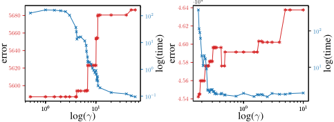
We investigated the influence of the parameter γ on the accuracy and runtime. The results are shown in Figure 1. The red curve corresponds to the change of errors as the increase of γ. The blue curve is for the change of the runtime.Observe that as the increase of γ, the error goes up from an optimal solution to a greedy solution, while the runtime decreases.
7 Conclusion
We study a common setting where several columns of one matrix are selected to simultaneously approximate all the columns of another matrix. While many algorithms were developed for the case where the target matrix has a single column, we are only aware of approximate algorithms for the general case. We observe that the general case cannot be reduced to the one column case, as the challenge is to select columns that approximate the entire target matrix.
The algorithms that we develop are similar to the (Weighted) A∗ algorithm. We show that with 0 assigned to a weight parameter, the algorithm is guaranteed to be optimal, but its running time may be very slow. Other nonzero choices give practical algorithms that beat the accuracy of the current state of the art algorithms.
In addition to producing a solution, our algorithms calculate bounds on how far the solutions are from the optimum. The quality of these bounds are data dependent. In some cases they provide no useful information, but in other cases it shows that the computed result is very close to the optimal solution. This is the case even for the greedy variant of our algorithm. It produces the same result as other known algorithms but gives the additional information of a bound.
While there is a significant similarity between our algorithm and the classical theory of the (Weighted) A∗ , we are not aware of direct applications of A∗ to the problem discussed here. In particular, our upper bound does not seem to have a parallel in the general theory.
@inproceedings{ijcai2021p221,
  title     = {Heuristic Search for Approximating One Matrix in Terms of Another Matrix},
  author    = {Wan, Guihong and Schweitzer, Haim},
  booktitle = {Proceedings of the Thirtieth International Joint Conference on
               Artificial Intelligence, {IJCAI-21}},
  publisher = {International Joint Conferences on Artificial Intelligence Organization},
  editor    = {Zhi-Hua Zhou},
  pages     = {1600--1606},
  year      = {2021},
  month     = {8},
  note      = {Main Track},
  doi       = {10.24963/ijcai.2021/221},
  url       = {https://doi.org/10.24963/ijcai.2021/221},
}
TY - CPAPER TI - Heuristic Search for Approximating One Matrix in Terms of Another Matrix AU - Wan, Guihong AU - Schweitzer, Haim T2 - Proceedings of the Thirtieth International Joint Conference on Artificial Intelligence, IJCAI-21 PB - International Joint Conferences on Artificial Intelligence Organization PY - 2021 SP - 1600 EP - 1606 DO - 10.24963/ijcai.2021/221 UR - https://doi.org/10.24963/ijcai.2021/221 ER -Copied
Machine-readable versions of this paper, for tools and AI agents:





