Knowledge-based Residual Learning

1 Introduction

Training with small number of data samples has always been one of the biggest challenge in machine learning. In many scientific domains, such as physics and environmental science [Karpatne et al., 2017b], sharing or obtaining data is often at a high cost. How to learn an accurate machine learning model from small data attracts many researchers.

In literature, people have tried to tackle this challenge in two major groups of approaches. The first group is transferring knowledge from other machine learning models to the target machine learning model. In this group, frequently used approaches include transfer learning [Pan and Yang, 2009], multi-task learning [Ranjan et al., 2019], and metalearning [Finn et al., 2017]. This group of approaches require data from the source domain or from other tasks in order to train machine learning models. It does not work for the case where there is a only one task with limited training data.

Another group of methods use domain expertise to tackle small data challenge. Frequently-used approaches include curating data representations [Khandelwal et al., 2015], changing loss functions [Karpatne et al., 2016a], and combining domain knowledge model with machine learning model [Ajay et al., 2019]. These approaches do not necessarily compete with each other and can be used at the same time.

∗ Part of the work was done when Guanjie Zheng was completing his PhD at the Pennsylvania State University.

In this paper, we focus on how to combine domain models with the machine learning models. We assume that there is a known domain knowledge model y = ρ(x) modeling the relation between features x and response variable y. We investigate this direction because from our collaborations with researcher from different disciplines such as environmental science and social science, we find that these researchers often know some simple model based on the scientific principles (e.g., physical laws or chemical reactions). Those domain knowledge models capture the correlations between features and target variable under the ideal assumptions. But the real world often violate the ideal assumptions, though the principles stay true. The actual models are often more complicated than the ones that domain experts have.

Different from the previously mentioned methods, we propose a surprisingly simple yet effective method to combine domain knowledge model and machine learning model. The key idea of our method is to treat the domain knowledge model as a weak learner and use the machine learning model (neural network is used) to learn the residual from the domain knowledge model. The idea is inspired by the boosting methods [Chen and Guestrin, 2016] and residual learning methods [He et al., 2016]. The key difference here is that our weaker learner is not a machine learning model, but a domain knowledge model derived by domain principles.

We further prove that the proposed hybrid model, when choosing neural network as the machine learning model, is guaranteed to outperform a pure neural net model and a pure domain knowledge model. We have conducted comprehensive experiments on real datasets from a variety of domains and have shown the superior performance of the proposed hybrid residual model. Case studies have shown how this method can boost the performance and maintain important domain properties. It demonstrates that our proposed hybrid residual model can help researchers in other disciplines to tackle their small data challenge.

2 RelatedWork

2.1 Combining Domain Knowledge Model and Machine Learning Model

This area has become increasingly popular recently [Karpatne et al., 2017a; Wagner and Rondinelli, 2016]. The most intuitive way is to use one component to help the other. (1)

[Chapelle and Li, 2011] use massive data to calibrate the domain knowledge model. (2) Domain knowledge can also be used in data preprocessing and postprocessing [Khandelwal et al., 2015]. However, these two categories of methods need a large amount of data for calibration or training. Hence, they do not apply to the small data problem mentioned before. In addition, they assume the domain model to be precise, which is usually not true.

Another idea is to integrate domain knowledge and machine learning models. (1) Many domain-specific machine learning model designs are proposed according to domain properties [Leibo et al., 2017; Mikolov et al., 2010], e.g., RNN structures [Mikolov et al., 2010] for natural language processing according to the sequential property. These methods are incorporating the specific domain properties, rather than the domain knowledge model in our problem. (2) Domain knowledge can also be used to guide the learning process as model initialization [Schrodt et al., 2015], regularization, priors or constraints [Karpatne et al., 2016b; Karpatne et al., 2016a]. These methods are usually sensitive to hyperparameter settings and performance of them vary among datasets. (3) Recently, several hybrid knowledge-data models are proposed [Ajay et al., 2019; Jia et al., 2019], such as using the output of one model (domain knowledge model or machine learning model) as features to the other model [Karpatne et al., 2017b]. Different from all the three categories of methods, we use the domain knowledge model as a weak learner and use a machine learning model (we use neural net) to boost it. This guarantees the superior performance of our model over either pure neural net model or domain knowledge model. We have tested its performance on routing problem in our earlier work [Liu et al., 2021].

2.2 Residual Learning and Boosting

Our method is related to boosting theory and residual learning theory. So we briefly review these studies. Boosting methods [Chen and Guestrin, 2016] serve as the state-of-the-art for many applications before recent deep learning methods. The success of boosting methods is attributed to their capability in ensembling weak learners and reducing bias [Chawla et al., 2003]. ResNet [He et al., 2016] is one essential advancement of deep learning. It enables multiple paths from input to output and resolves the gradient vanishing problem. It significantly improves the performance of deep learning methods on supervised learning tasks, e.g., image classification [He et al., 2016], and spatial-temporal prediction [Liu et al., 2019]. Recent research has explored the connection between ResNet and boosting theory. [Huang et al., 2017] have demonstrated that ResNet can be regarded as the ensemble of multiple paths from input to output, and has shown ResNet can be learned in a boosting way.

In contrast, we propose a hybrid framework, which incorporates domain knowledge in a residual learning way. The domain knowledge model serves as the skip connection in ResNet, or a weak learner in boosting theory. This connection guarantees the success of the proposed framework.

3 ProblemDefinition

Our problem definition follows typical regression and classification problem definition. Specifically, we are given a dataset of N data points. Each data point, represented as (xi, yi), is composed of a feature vector xi ∈ Rd and a response value yi ∈ R (for regression) or yi ∈ {0, 1, ..., K-1} (for classification). Domain knowledge model is given as yD = ρ(x). Our problem can be formulated as follows:

Problem 1 (Domain-Aware-Prediction). Given a dataset {(x1, y1), (x1, y2), ..., (xN, yN)}, and domain knowledge model yD = ρ(x), the goal is to build a prediction model y = F(x, ρ(x)), so that the defined loss is minimized.

4 Method

To tackle the aforementioned challenges of small data, we propose a Knowledge-based Residual Learning method (KRL). This model is composed of domain knowledge model part and neural net part.

4.1 Combining Domain Knowledge Model and Machine Learning Model

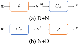
Here, we show two intuitive combinations of domain knowledge and neural network models (as in Figure 1). Some studies [Wilby et al., 1998] stack domain knowledge model output to a neural network to predict the response (Figure 1 (a)). This design enables fine-tuning towards the correct scaling over the domain knowledge model output. Some other studies [Sadowski et al., 2016] preprocess the data by a neural network and feed to domain knowledge model (Figure 1 (b)). This helps de-noise the input and get better prediction y through domain knowledge model. These designs require the special form of the domain knowledge model, and lead to inferior performance when domain knowledge has flaw.

4.2 Residual Learning for Knowledge-Data Hybrid Model

Inspired by the observation that domain knowledge model can capture a rough mapping between feature and response,

<

l

a

t

e

x

i

s

h

1

_

b

6

4

=

"

z

3

W

N

G

Z

y

f

5

D

u

7

L

E

R

w

V

C

T

A

>

B

8

n

c

S

g

M

F

U

2

v

q

k

K

j

0

X

9

H

o

Y

+

d

m

Q

r

/

I

p

P

O

J

<

l

a

t

e

x

i

s

h

1

_

b

6

4

=

"

z

3

W

N

G

Z

y

f

5

D

u

7

L

E

R

w

V

C

T

A

>

B

8

n

c

S

g

M

F

U

2

v

q

k

K

j

0

X

9

H

o

Y

+

d

m

Q

r

/

I

p

P

O

J

<

l

a

t

e

x

i

s

h

1

_

b

6

4

=

"

Z

/

f

p

B

q

r

z

c

d

S

Y

K

P

n

5

v

D

8

>

A

7

3

V

N

E

J

W

X

O

k

9

F

j

0

o

M

g

U

T

m

G

H

2

+

Q

u

w

L

I

R

C

y

<

l

a

t

e

x

i

s

h

1

_

b

6

4

=

"

9

w

f

d

L

R

B

j

C

k

y

T

3

Y

5

p

2

g

Q

>

A

c

V

D

S

N

E

O

z

G

M

r

H

8

0

o

W

I

+

U

v

m

/

K

u

7

Z

q

J

X

n

F

P

<

l

a

t

e

x

i

s

h

1

_

b

6

4

=

"

m

X

c

f

0

5

P

C

z

L

u

/

W

v

>

A

B

7

n

V

N

S

w

M

E

J

2

+

T

R

p

F

Y

9

O

K

g

d

3

Z

G

r

y

Q

I

H

j

o

D

k

8

q

U

<

l

a

t

e

x

i

s

h

1

_

b

6

4

=

"

p

X

F

W

G

y

N

k

r

S

K

q

D

E

5

2

f

g

Q

R

w

c

>

A

B

8

n

V

L

M

3

P

d

m

Z

Y

u

U

z

v

j

o

0

7

/

O

H

9

J

I

T

C

+

<

l

a

t

e

x

i

s

h

1

_

b

6

4

=

"

Z

/

f

p

B

q

r

z

c

d

S

Y

K

P

n

5

v

D

8

>

A

7

3

V

N

E

J

W

X

O

k

9

F

j

0

o

M

g

U

T

m

G

H

2

+

Q

u

w

L

I

R

C

y

<

l

a

t

e

x

i

s

h

1

_

b

6

4

=

"

9

w

f

d

L

R

B

j

C

k

y

T

3

Y

5

p

2

g

Q

>

A

c

V

D

S

N

E

O

z

G

M

r

H

8

0

o

W

I

+

U

v

m

/

K

u

7

Z

q

J

X

n

F

P

<

l

a

t

e

x

i

s

h

1

_

b

6

4

=

"

m

E

c

z

F

L

u

G

B

p

P

5

0

q

A

I

J

g

>

H

V

N

S

8

3

U

r

/

9

o

M

2

Q

+

D

Z

j

Y

w

y

f

d

W

X

7

v

C

k

K

T

n

R

O

<

l

a

t

e

x

i

s

h

1

_

b

6

4

=

"

m

E

c

z

F

L

u

G

B

p

P

5

0

q

A

I

J

g

>

H

V

N

S

8

3

U

r

/

9

o

M

2

Q

+

D

Z

j

Y

w

y

f

d

W

X

7

v

C

k

K

T

n

R

O

we propose a residual learning method to combine domain knowledge and neural net model. Generally, one classic residual unit can be defined as

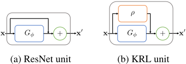
where Gφ is an arbitrary neural net, and H(x) is a skip connection (e.g., a simpler neural layer). A fully-connected layer is usually added after the final residual unit to map x′ to y. By setting H(x) as identity mapping, we have the widelyused form x′ = x+Gφ(x) (as in Figure 2 (a)).

Studies have revealed two reasons that make ResNet successful: (1) Learning the residual value y′ - y is provable better than learning original value y when Gφ satisfies certain criteria and output layer is linear [Shamir, 2018]. (2) The shortcut link x creates O(2n ) paths from the input to the output when n residual layers stack together [Veit et al., 2016]. This ensemble significantly increases its robustness and accuracy.

Hence, we propose a simple but effective residual unit with domain knowledge (as in Figure 2 (b))

where ρ(x) is the domain knowledge model, Gφ(x) is a neural net model. Intuitively, the domain knowledge model can predict the data reasonably well. Hence, the neural net model will be directed to predict the residual x′ - ρ(x). Moreover, theoretically, it is guaranteed to yield superior performance over either pure domain knowledge model or pure deep learning model (shown in the next section).

4.3 Performance Guarantee

Guarantee to Outperform Domain Knowledge Model

Without loss of generality, we can assume the final output layer as

where x is the output from the previous residual unit, w is linear weight vector, ρ is the domain knowledge model and Gφ is a neural net. Further, we can re-write Eq. (3) as follows by explicitly write out the last fully-connected layer M

Then, setting M equal to 0, the domain knowledge model is represented as

Next, we will prove that the hybrid model Eq. (4) will perform not worse than the domain knowledge model Eq. (5). Before that, we need to incorporate the following general version corollary from [Shamir, 2018] (this corollary can be proved in the exactly same fashion as the Corollary 1 in [Shamir, 2018] by replacing the identity mapping with more general version, a differentiable function H(x)).

Corollary 1. Suppose we have a function defined as

where l is the defined loss, a, B are weight vector and matrix respectively, and ψ is the parameters of a neural network. Then, every local minimum of Γ satisfies

if the following two conditions are satisfied: (1) loss l(ˆ y, y) is twice differentiable and convex in ˆ y; (2) Γψ(a,B), ▽Γψ(a,B), and ▽2Γψ(a,B) are Lipschitz continuous in (a, B).

Then, we can prove the following theorem (please see appendix for details) 1 .

Theorem 1. When using squared loss (for regression) and exponential loss or logistic loss (for classification), every local optimum of hybrid model y = wT (ρ(x) +MGθ(x)) will be not worse than domain model y = wT ρ(x).

Guarantee to Outperform Neural Net Model

By further building connection with boosting theory [Huang et al., 2017], we will prove that KRL outperforms pure neural net model. Here, we use binary classification as an example. For the convenience of derivation, we apply exponential loss following the convention in the boosting theory. This derivation can be extended to logistic loss. The derivation for regression is left to future work.

First, we need to incorporate a corollary about AdaBoost. When using the exponential loss function L(y, f(x)) = exp(-yf(x)), the objective of AdaBoost algorithm can be written as

where m is the index of the weak learner. Then, the following corollary has been proved in [Hastie et al., 2009].

Corollary 2. With exponential loss function, the AdaBoost algorithm is equivalent to forward stagewise additive modeling, and the classification error is guaranteed to decay when the number of base learners increase. The objective Eq. (8) can be achieved by solving the Gm and βm sequentially.

Thus, we can have the following corollary.

Corollary 3. Given Gm, the classifier obtained by the following objective is guaranteed to reduce the loss compared with fm-1(x).

Then, we can prove the following theorem (please see appendix for details).

Theorem 2. The hybrid model y = wT (ρ(x) + Gφ(x)) is guaranteed to reach a minimum not worse than the pure neural net model y = wT 1 Gφ(x).

5 Experiment

5.1 Experiment Settings

We conducted experiments on the following domains, covering regression, classification and information retrieval (IR) problems. Details and citations of the datasets can be found in the supplementary materials.

1 The appendix will be released on the authors' website and arxiv.

Table 1: Overall performance comparison."-" means the method does not apply to this dataset. ↑ means the higher the better and ↓ means the lower the better. Some methods perform similar on certain datasets because of the float precision. We show the average results of 5 runs.

Method		Regression (RMSE↓)				Classification (Accuracy↑)	IR (F1↑)
		Weather	Radi	Pend	Spring	Loan	Routing
Domain	DOM	102.48	3.1	1.1	0.47	0.51	0.64
Machine	Ridge	368.56	3.99	0.72	0.38	-	-
	XGBoost	464.73	3.79	1.84	0.71	0.54	0.09
	LR	-	-	-	-	0.54	0.22
learning	NN	746.19	2.93	0.57	0.39	0.55	0.22
	ResNet	720.82	3.52	0.66	0.67	0.54	0.22
Hybrid	LfD	833.84	2.82	0.53	0.39	0.55	0.21
	N+D	975.69	2.96	0.82	0.4	0.51	-
	D+N	113.07	2.91	0.86	0.53	0.55	0.64
	RF-D	104.36	2.45	0.56	0.4	0.55	0.53
	D-Cons	735.48	2.63	0.64	0.38	0.51	0.22
	KRL	100.48	2.23	0.47	0.35	0.57	0.76

• Weather [Brantley et al., 2008]. This dataset documents the soil formation and weathering process of chemicals in soils. It contains 178 records at various depths. We use the soil depth from the ground surface and time to predict chemical concentrations in the soil. For the domain knowledge model, a sigmoid-family analytical equation [Brantley et al., 2008] describing the relation between chemical concentration and depth is utilized.
• Radi [TEPCO, 2019]. This dataset has 3,371 concentration samples of multiple radiative chemical analytes in the seawater near Fukushima Daiichi Nuclear Power Station since the nuclear disaster. We use the time as the feature to predict the remaining percentage of the concerned analyte. The radioactive decay rate equation [Bucknell, 2019] (as shown in 10) is included as the domain knowledge model.

Here, N and N0 are the analyte concentration at time t and time t = 0 respectively, and λ is the decay constant.

• Pend [Greydanus et al., 2019]. This dataset describes the Hamiltonian dynamics of a pendulum system. Hamiltonian mechanics defines coordinates (e.g., position, momentum) to describe the system. For instance, an ideal pendulum system can be described by the following equation [Greydanus et al., 2019].

Here, p, q are the coordinates (position and momentum correspondingly), and H is the Hamiltonian of this system. Additionally, m, l represent the mass and length of the pendulum respectively, and g is the gravity constant. Then, the system dynamics (w.r.t. time) can be described by the derivative of the coordinates. We use the coordinates to predict the changing rate of these coordinates w.r.t. time.

• Spring [Greydanus et al., 2019]. This dataset describes the Hamiltonian dynamics of a spring system. Ideally, this system can be described by the following formula

• where m is the mass of the spring, and k is the spring constant. Similar as in Pend, the two coordinates are used to predict the changing rate of the defined coordinates. The analytical equation for this spring system is used as the domain knowledge model.
• Routing [Moreira-Matias et al., 2013]. This dataset contains 7,734 pieces of taxi trajectories in Porto, Portugal from July 1, 2013 to June 30, 2014. We use the central business area (with 69 intersections) of Porto to build a weighted graph, and then use the origin, destination and departure time information to predict the routes of the vehicles (represented as a vector of 0 and 1 with each bit stand for one road segment). This problem is similar to an information retrieval problem. We use Dijkstra algorithm as the domain knowledge model to find the shortest path. For specific implementation details, please refer to this work [Liu et al., 2021] we finished earlier.
• Loan [Kaggle, 2019]. This dataset contains vehicle loan records. Each record contains features of the borrowers (e.g., employment status, credit history), loan amount, and whether default happened. We aim to predict the default (0 or 1) and utilize the exponential utility function as the domain knowledge.

5.2 ComparedMethods

We compare with three groups of methods, domain models (DOM), machine learning models (LR: Logistic Regression, Ridge: Ridge Regression, XGBoost [Chen and Guestrin, 2016], NN: neural net, ResNet [He et al., 2016]) and hybrid models as follows. By default, all neural net models are composed of 3 hidden layers with 32 neurons.

• LfD [Argall et al., 2009]: Learning from demonstration. This method first generates some data from the domain knowledge model and train a neural net model with both generated data and original data.
• D+N [Wilby et al., 1998]: This method feeds the output from a domain knowledge model to a neural net. This

allows fine-tuning of the scale of the output from domain knowledge model.

• N+D [Sadowski et al., 2016]: This method first uses a neural net to map the raw features to the input of the domain knowledge model. The output from the domain knowledge model is the final prediction.
• RF-D [Wang et al., 2017] utilizes a random forest based method to predict the discrepancy between the domain knowledge model output and the observation.
• D-Cons [Karpatne et al., 2016b] uses domain knowledge as a constraint (i.e., an auxiliary loss) to the main loss.
• KRL: We propose a residual learning framework to combine the domain knowledge and the machine learning model. We name the method as KRL (Knowledge-based Residual Learning).

5.3 RQ1: Overall Prediction Accuracy

To verify the effectiveness of KRL, we conduct experiments on multiple datasets (results shown in Table 1). As expected, our proposed method KRL outperforms all the baselines on all datasets. Interestingly, the Hybrid group of methods usually achieves better results than other methods. Further, despite the unstable performance of other Hybrid methods, KRL consistently performs the best.

5.4 RQ2: How the Domain Knowledge Helps

Robust Mimicking from Domain Knowledge Model

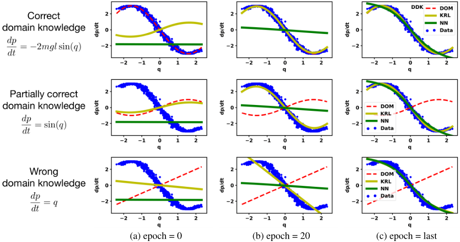
We investigate a pendulum system [Greydanus et al., 2019] with mass m and length l, and collect the data and model fitting results during the training process. This system is described by Hamiltonian Dynamics, where two variables p, q are defined to represent the position and the momentum of the pendulum respectively. Different models (KRL, NN) are built to capture the mapping between q(position change rate) and dp/dt(time).

When the correct domain knowledge is incorporated (first row in Figure 3), KRL can better predict the response and converge faster (at epoch 20). Specifically, KRL can learn the sine function relation but NN can not (even at the last epoch). When a partially correct formula is provided (second row in Figure 3), KRL can still learn the correct response. Even with a totally wrong formula (third row in Figure 3), KRL is able to abandon the wrong formula and converge to similar results as pure data-driven model NN. Thus, KRL can utilize the correct information in the domain knowledge model to converge to a better result faster, and avoid mistakes in the domain knowledge model.

Maintaining Domain Properties

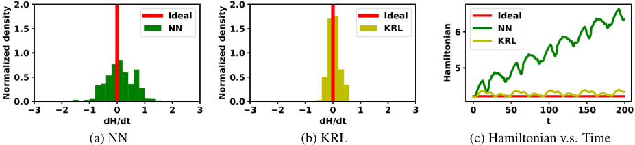
Incorporating domain knowledge model also enables the learned model to maintain domain properties. Following the setting in the previous experiment, we show how the Hamiltonian changes over time in this system. The Hamiltonian of this system is supposed to keep constant (i.e., dH/dt always equals 0) because it is energy loss-free. As shown in Figure 4, in the results recovered by NN (Figure 4 (a)) dH/dt can vary in a relatively large range, while in the results recovered by KRL (Figure 4 (b)) dH/dt remains close to 0. In addition, when using the predicted dp/dt and dq/dt to control the system (Figure 4 (c)), the system controlled by KRL successfully keeps the Hamiltonian stable though small variation is observed, while the system controlled by NN experiences an explosion of Hamiltonian, which is impossible in reality.

6 Conclusion

In this paper, we propose to solve the limited data issue for real world problems by incorporating domain knowledge. We propose a model KRL, and prove that the proposed model has a guaranteed superior performance over the domain knowledge model and pure neural net. Extensive experiments are conducted and have shown the superior performance of KRL over baselines. We have also demonstrated the domain knowledge can help maintaining domain properties.

Our proposed model can be extended to various kinds of problems, and incorporated in different model designs. We believe it will be a general and essential progress in the application of machine learning models for real world problems where data is limited but the mechanisms are complex.

Acknowledgments

This work was supported in part by NSF awards #1652525, #1618448 and #1639150. The views and conclusions contained in this paper are those of the authors and should not be interpreted as representing any funding agencies.