
Inferring Time-delayed Causal Relations in POMDPs from the Principle of Independence of Cause and Mechanism
Proceedings of the Thirtieth International Joint Conference on Artificial Intelligence. Main Track. Pages 1944-1950.
https://doi.org/10.24963/ijcai.2021/268
Keywords
- Knowledge Representation and Reasoning: Action, Change and Causality
- Robotics: Cognitive Robotics
Abstract
This paper introduces an algorithm for discovering implicit and delayed causal relations between events observed by a robot at regular or arbitrary times, with the objective of improving data-efficiency and interpretability of model-based reinforcement learning (RL) techniques. The proposed algorithm initially predicts observations with the Markov assumption, and incrementally introduces new hidden variables to explain and reduce the stochasticity of the observations. The hidden variables are memory units that keep track of pertinent past events. Such events are systematically identified by their information gains. A test of independence between inputs and mechanisms is performed to identify cases when there is a causal link between events and those when the information gain is due to confounding variables. The learned transition and reward models are then used in a Monte Carlo tree search for planning. Experiments on simulated and real robotic tasks, and the challenging 3D game Doom show that this method significantly improves over current RL techniques.
- [Battaglia et al., 2016] Peter W. Battaglia, Razvan Pascanu, Matthew Lai, Danilo Jimenez Rezende, and Koray Kavukcuoglu. Interaction networks for learning about ob- jects, relations and physics. In Advances in Neural In- formation Processing Systems 29: Annual Conference on Neural Information Processing Systems 2016, December 5-10, 2016, Barcelona, Spain, pages 4502-4510, 2016.
- [Boots et al., 2011] Byron Boots, Sajid M Siddiqi, and Ge- offrey J Gordon. Closing the learning-planning loop with predictive state representations. Int. J. Rob. Res., 30(7):954-966, June 2011.
- [Boularias and Chaib-draa, 2009] Abdeslam Boularias and Brahim Chaib-draa. Predictive representations for policy gradient in pomdps. In Proceedings of the 26th Annual International Conference on Machine Learning, ICML, pages 65-72, 2009.
- [Chiappa et al., 2017] Silvia Chiappa, Sébastien Racaniere, Daan Wierstra, and Shakir Mohamed. Recurrent environ- ment simulators. arXiv preprint arXiv:1704.02254, 2017.
- [Choromanski et al., 2018] Krzysztof Choromanski, Carlton Downey, and Byron Boots. Initialization matters: Orthog- onal predictive state recurrent neural networks. In Pro- ceedings of the Sixth International Conference on Learn- ing Representations (ICLR), 2018.
- [Daniušis et al., 2010] Povilas Daniušis, Dominik Janzing, Joris Mooij, Jakob Zscheischler, Bastian Steudel, Kun Zhang, and Bernhard Schölkopf. Inferring deterministic causal relations. In Proceedings of the Twenty-Sixth Con- ference on Uncertainty in Artificial Intelligence, UAI'10, pages 143-150, 2010.
- [Diuk et al., 2008] Carlos Diuk, Andre Cohen, and Michael L. Littman. An object-oriented representation for efficient reinforcement learning. In Proceedings of the 25th International Conference on Machine Learning, ICML '08, pages 240-247, 2008.
- [Downey et al., 2017] Carlton Downey, Ahmed Hefny, Boyue Li, Byron Boots, and Geoffrey J. Gordon. Pre- dictive state recurrent neural networks. In Proceedings of Advances in Neural Information Processing Systems (NIPS), 2017.
- [Finn and Levine, 2017] C. Finn and S. Levine. Deep visual foresight for planning robot motion. In 2017 IEEE Inter- national Conference on Robotics and Automation (ICRA), pages 2786-2793, May 2017.
- [Finn et al., 2016] Chelsea Finn, Xin Yu Tan, Yan Duan, Trevor Darrell, Sergey Levine, and Pieter Abbeel. Deep spatial autoencoders for visuomotor learning. 2016 IEEE International Conference on Robotics and Automation (ICRA), pages 512-519, 2016.
- [Hafner et al., 2019] Danijar Hafner, Timothy Lillicrap, Ian Fischer, Ruben Villegas, David Ha, Honglak Lee, and James Davidson. Learning latent dynamics for planning from pixels. In International Conference on Machine Learning, pages 2555-2565. PMLR, 2019.
- [Kansky et al., 2017] Ken Kansky, Tom Silver, David A. Mély, Mohamed Eldawy, Miguel Lázaro-Gredilla, Xinghua Lou, Nimrod Dorfman, Szymon Sidor, D. Scott Phoenix, and Dileep George. Schema networks: Zero-shot transfer with a generative causal model of intuitive physics. In Proceedings of the 34th International Con- ference on Machine Learning, ICML 2017, Sydney, NSW, Australia, 6-11 August 2017, pages 1809-1818, 2017.
- [Kempka et al., 2016] Michal Kempka, Marek Wydmuch, Grzegorz Runc, Jakub Toczek, and Wojciech Jaskowski. Vizdoom: A doom-based AI research platform for visual reinforcement learning. CoRR, abs/1605.02097, 2016.
- [Kimmel et al., 2019] Andrew Kimmel, Avishai Sintov, Jun- tao Tan, Bowen Wen, Abdeslam Boularias, and Kostas E. Bekris. Belief-space planning using learned models with application to underactuated hands. In International Sym- posium on Robotics Research (ISRR), 2019.
- [Li et al., 2017] Yuezhang Li, Katia Sycara, and Rahul Iyer. Object-sensitive deep reinforcement learning. In Christoph Benzm\"uller, Christine Lisetti, and Martin Theobald, editors, GCAI 2017. 3rd Global Conference on Artificial Intelligence, volume 50 of EPiC Series in Com- puting, pages 20-35. EasyChair, 2017.
- [Mnih et al., 2013] Volodymyr Mnih, Koray Kavukcuoglu, David Silver, Alex Graves, Ioannis Antonoglou, Daan Wierstra, and Martin Riedmiller. Playing atari with deep reinforcement learning. arXiv:1312.5602, 2013.
- [Oh et al., 2015] Junhyuk Oh, Xiaoxiao Guo, Honglak Lee, Richard L. Lewis, and Satinder P. Singh. Action- conditional video prediction using deep networks in atari games. In NIPS, pages 2863-2871, 2015.
- [Rabiner, 1990] Lawrence R. Rabiner. Readings in speech recognition. chapter A Tutorial on Hidden Markov Models and Selected Applications in Speech Recognition, pages 267-296.
- [Scholz et al., 2014] Jonathan Scholz, Martin Levihn, Charles Isbell, and David Wingate. A physics-based model prior for object-oriented mdps. In Eric P. Xing and Tony Jebara, editors, Proceedings of the 31st International Conference on Machine Learning, volume 32 of Proceed- ings of Machine Learning Research, pages 1089-1097, Bejing, China, 22-24 Jun 2014.
- [Singh et al., 2004] Satinder Singh, Michael R. James, and Matthew R. Rudary. Predictive state representations: A new theory for modeling dynamical systems. In Proceed- ings of the 20th Conference on Uncertainty in Artificial Intelligence, UAI '04, pages 512-519, Arlington, Virginia, United States, 2004. AUAI Press.
- [Usunier et al., 2016] Nicolas Usunier, Gabriel Synnaeve, Zeming Lin, and Soumith Chintala. Episodic exploration for deep deterministic policies: An application to starcraft micromanagement tasks. CoRR, abs/1609.02993, 2016.
- [Vaswani et al., 2017] Ashish Vaswani, Noam Shazeer, Niki Parmar, Jakob Uszkoreit, Llion Jones, Aidan N Gomez, Łukasz Kaiser, and Illia Polosukhin. Attention is all you need. In Advances in neural information processing sys- tems, pages 5998-6008, 2017.
- [Wang et al., 2017] Zhikun Wang, Abdeslam Boularias, Katharina Muelling, Scholkopf Bernhard, and Jan Peters. Anticipatory action selection for human-robot table tennis. Artificial Intelligence, February 2017.
References were extracted automatically from the PDF and may contain errors.
Full text extracted automatically from the PDF; figures, tables and equations may differ. The PDF is the version of record.
1 Introduction
Despite the remarkable progress made by deep RL agents in reaching human-level performance and beyond [Mnih et al., 2013], they continue to lag behind humans in terms of data efficiency. Humans can immediately figure out the effects of their actions on objects displayed on a screen after a few trials, and build a model for reasoning and planning in order to improve their scores. Model-based RL algorithms arguably require less data than model-free ones [Hafner et al., 2019; Finn et al., 2016; Finn and Levine, 2017]. But learning models that are sufficiently accurate for planning is still a challenging problem [Battaglia et al., 2016]. Inaccurate predictions generally result in sub-optimal policies.
The difficulty in learning accurate predictive models can be mostly attributed to the partial observability of the states. In robotics, for example, the Markov condition is seldom verified [Wang et al., 2017; Kimmel et al., 2019]. Future states and rewards often depend on the entire history of actions and observations. An example of that is unlocking a door and opening it afterwards. The first action changes the hidden variable that is the state of the door from locked to unlocked. Without a memory of past locking/unlocking actions, a robot cannot explain why the door opens sometimes and does not open other times based only on an image of the door. The robot needs to infer the hidden causal link between the act of unlocking the door and the ability to open it later in the future. Other examples include filling or pouring liquids from containers, turning electric switches and unscrewing a lid and lifting it later in the future. In general, sequential object manipulation tasks involve changing states of objects in ways that cannot be easily perceived through vision, but their effects can be observed in the later stages of the task.
LSTM and GRU architectures are general-purpose tools for solving problems of partial observability by discovering and remembering pertinent information. They tend, however, to require large amounts of data, and they cannot be easily interpreted. To address these two issues, we present here an approach that combines the merits of general function approximators such as neural networks with probabilistic graphical models for representing hidden variables. Given a stream of actions, observations and rewards, a neural network is trained to predict future observations and rewards. Simultaneously, a graphical model of causal relations between observations occurring at different time steps is also gradually constructed. The values of the variables in the graph are also provided to the neural network as additional inputs along with the observations. The learned predictive model is then utilized by the agent to select actions based on their predicted future rewards.
2 Background and Notations
Formally, a Markov Decision Process (MDP) is a tuple (S, A, T, R, γ), where S is a set of states and A is a set of actions. T is a transition function with T(s′ |a, s) = P(St+1 = s′ |St = s,At = a) for s, s′ ∈ S, a ∈ A, and R is a reward function where R(s, a, r) is the probability of receiving reward r ∈ R for executing a in s. A policy π is a distribution on the action to be executed in each state, defined as π(s, a) = P(at = a|st = s). The value V π of a policy π is the expected sum of rewards that will be received if π is followed, i.e., V π (s) = E[∑∞t=0 γ t rt|S0 = s, π, T, R].
In video games and robotics, states generally cannot be fully observed. Instead, the agent perceives partial observations zt, in the form of images, for example. The resulting process is a Partially Observable MDP (POMDP). Formally, a POMDP is a tuple (S,A,Z, T, F,R, γ) where (S,A, T,R, γ) is an MDP, Z is a set of observations, and F is an observation likelihood function: F(Z|S) is the probability of observing Z ∈ Z in state S ∈ S.
We focus in this work on object-oriented POMDPs, where a state S is described by one or several visible attributes of objects, in addition to one or several hidden variables. In other terms, S = (O1 ,O2 , . . . ,On ,M 1 ,M 2 , . . . ,M m) ∈ ∏ni=1 Oi × ∏mi=1 Mi, wherein Oi is an attribute of an object in the scene, and M i is a hidden variable. The list of objects includes the robot or its end-effector. Oi andMi denote the domains of visible variable Oi and hidden variable M i , respectively, which can be discrete or continuous. For example, O1 is the position of a specific object in the image, while O2 is its velocity, O3 is its size, O4 is its numerical label, O5 is a Boolean attribute that indicates if the object still exists in the scene or not, O5 is the position of a second object in the image, and so forth. Observations correspond to object attributes, i.e., Zt = (Oi t )ni=1 . To ease the notation, we also consider the reward signal Rt as one of the observable attributes Oi t . Thus, the reward function is modeled and learned in the same way as the transition function. We focus hereafter on the general problem of predicting future states.
Hidden variables M 1 ,M 2 , . . . ,M m are unknown a priori and need to be inferred from the observable entities. Examples of hidden variables M i include past events, or actions performed on the objects. In the previous example, a door can be unlocked or locked at a given time t, and the state of the door cannot be easily inferred from vision alone. The state of the door is then a hidden variable M i t of state St . Its existence can be inferred by discovering the causal link between the act of inserting and turning a key in a door lock and the subsequent ability to open the door later in the future, after executing several possibly unrelated actions. Transition function T is represented as a Dynamic Bayesian Network (DBN). We denote by pa(Xt) the list of parents of variable X at time t. Thus, function T is defined as T(St+1|St,At) = ( ∏ni=1 P (Oi t+1|pa(Oi t+1), At))( ∏mi=1 P (M i t+1|pa(M i t+1), At)), wherein the values of Oi t+1 andM i t+1 are contained in St.
3 RelatedWorks
The Baum-Welch algorithm is an expectation-maximization technique that is traditionally used to learn hidden Markov models and POMDPs [Rabiner, 1990]. This algorithm requires knowing the number of hidden variables in advance. It is sensitive to the initial values of parameters and typically results in suboptimal solutions. Predictive state representations (PSRs) [Singh et al., 2004] are an alternative model to represent partially observable environments without using hidden states. While parameters of PSRs can be learned with any consistent density estimator, discovering the core tests is still an open problem. Moreover, the learning complexity of these estimators is exponential in the length of history that needs to be stacked to predict future observations [Boularias and Chaib-draa, 2009]. A more efficient spectral approach proposed in [Boots et al., 2011] generalizes PSRs by including features of test outcomes and histories, instead of a stream of raw observations. For example, an indicative feature might be the number of times we saw a specific observation in the past three steps. The memory variables introduced in the present work are closely related to the indicative features. In contrast to [Boots et al., 2011], our algorithm reasons about the causal relations between different regions of the observation space and over different time intervals, and returns an explicit graphical representation of the discovered causal relations. Most recent efforts on learning partially observable dynamical models rely on recurrent neural networks (RNN) and LSTM techniques [Downey et al., 2017; Choromanski et al., 2018; Hafner et al., 2019; Finn and Levine, 2017; Finn et al., 2016]. While the success of LSTM is not fully understood, it is frequently attributed to the gating mechanisms that allows information to be retained for a long time, but also to be forgotten quickly.
In vision-based RL, there is a clear physical structure that can readily be exploited. Images can be decomposed into segments of objects. Several models utilizing object-oriented representations for learning and planning have been proposed in the past [Diuk et al., 2008; Scholz et al., 2014; Usunier et al., 2016]. Object-sensitive deep RL is a closely related idea proposed in [Li et al., 2017]. More recent works focused on learning these models, such as the interaction networks [Battaglia et al., 2016; Kansky et al., 2017], which can reason about how objects in complex systems interact.
4 Proposed Approach
The proposed approach initially assumes that there are no hidden variables, and incrementally creates new ones only when needed to explain stochasticity of outputs. Algorithm 1 summarizes the main steps of this process.
4.1 Identifying Highly Stochastic Variables
We start by setting m, the number of hidden variables, to 0, and initialize the list of parents pa(Oi t+1 ) with {O1 t , . . . ,On t ,At}. In other words, all attributes of objects in a given state are considered as relevant for predicting the next state. Next, factors P(Oi t |pa(Oi t )) of the transition function are estimated from trajectories D. This can be achieved through any of the many existing density estimation techniques, such as frequency counts of discretized variables.
The algorithm maintains an open last-in, first-out list that contains state variables that need further explanation, i.e., variables with probability distributions that have an entropy above a predefined threshold ϵ. The algorithm is safeguarded against entering infinite loops by upper bounding the number of parents per variable by max var. The algorithm processes the variables, one at a time, until the open list is empty.
4.2 Searching For Possible Causes Of Uncertainty
For each variable X in the open list, we identify a second variable Y that yields the highest information gain when utilized along with the current parents of X to predict X (line
9). The question that we want to answer here is: Does knowing the value of Y at time t + τ help us predict the value of X at time t? Here, τ is a shift in time that takes values from [τ -, τ +], wherein τ - < 0 and τ + ≥ 0 and the choice of τ - and τ + depends on the computational resources that are available and the amount of data. Notice that τ = -1 can be excluded from the interval because Yt-1 is already a parent of Xt (line 3). The interval of time shifts τ includes positive values as well because we are also interested in finding links between Xt and future values of variable Y . We will return to this specific point later.
We found from our experiments that adding together the information gains of Yt+τ for different values of τ results in a better detection of relations between X and Y , given that the delays in these relations can be arbitrary long. In the previous example, the robot may unlock the door then performs a large number of unrelated exploratory actions before opening it. The time difference τ between the first event of unlocking the door and the second one of opening the door is arbitrary large. The first event is captured by a variable Y that indicates the position of the key relative to the doorknob, and the second event is captured by a Boolean variable X. To explain why Xt takes values from the set {open, closed} randomly when conditioned on the action and attributes at time t - 1, the algorithm identifies Y as a potential cause by noticing the information gain of adding Yt+τ to Xt's parents, for τ ∈ [τ -, -1[∪]-1, τ +]. Information gain and conditional entropy are approximated empirically by replacing expectations with averages computed from the training data.
4.3 CreatingMemories Of Identified Causes
Once a variable Y is selected as a new parent of X, we search in the space Y of all possible values that Y can take for the ones that are affecting X's distribution the most. Note that if all values of Y turn out to be relevant to the prediction of X then they will all eventually be selected, as long as their number does not exceed the upper bound max var. For computational efficiency, the space Y of variable Y is recursively divided into different regions by using the binary space partitioning (BSP) technique (line 10). For example, if Y is the 3D position of the robot's end-effector relative to a door knob, then Partition(Y) is an octree.
In the next steps (lines 11-14), a memory of visiting a region ¯ Y is created for every possible region in the partition of Y 's domain. The memory variable is denoted by M¯ Y. It is indexed by ¯ Y because it serves as a timer that indicates the time elapsed since the most recent time when state variable Y took a value from the set ¯ Y, i.e., Y ∈ ¯ Y. Thus, the domain of M¯ Y , denoted by M ¯ Y, is set as [-1,∞[. Default valueM¯ Y,t = -1 means that, up to time t, the event Y ∈ ¯ Y did not occur yet. The parents of M¯ Y,t are M¯ Y,t-1 and Yt. Memory variable M¯ Y is simply a timer that is set to 0 the moment the event Yt ∈ ¯ Y occurs, and that is incremented by 1 every time-step afterwards. Instead of retaining all memory variables M¯ Y for all possible regions ¯ Y of Y 's domain, we choose in this work to retain only a specific memory M¯ Y that corresponds to the region ¯ Y that brings the maximum information gain to the prediction of X (line 15).
Algorithm 1: Greedy Causal Graph Construction
Input: Set of observable variables {Oi }ni=1, and sampled data trajectories D = {(zl0, al0, . . . , zlh, alh)}Ll=1; Output: Set of memory variables {M i }mi=1, and parents of each variable in {M i }mi=1 ∪ {Oi }ni=1 ; 1 openList ← ∅; m← 0; /* Identifying stochastic variables */ 2 for i := 1; i ≤ n; i ← i +1 do 3 ∀t ≥ 0 : pa(Oi t+1) ← {O1 t , . . . ,On t ,At}; 4 Estimate P(Oi t |pa(Oi t)) from data D; 5 if ConditionalEntropy(Oi , pa(Oi ),∅)≥ ϵ then openList.push(Oi ) ; 6 while openList ̸= ∅ do 7 X ← openList.pop(); newParents ← ∅; /* Searching causes of uncertainty */ 8 repeat 9 Y ← argmax Y ∈{Mi}mi=1 ∪{Oi}ni=1 τ +∑ τ=τh∑ t=0 InfoGain(Xt, Yt+τ) ; 10 foreach ¯ Y ∈ Partition(Y) do /* Creating memories */ 11 M¯ Y ← [-1,∞[; pa(M¯ Y,t+1) ← {M ¯ Y,t, Yt}; P (M ¯ Y,0 = -1) = 1; 12 if (Yt ∈ ¯ Y) then P (M ¯ Y,t+1 = 0|pa(M¯ Y,t+1)) = 1 ; 13 if (Yt /∈ ¯ Y) ∧ (M ¯ Y,t ≥ 0) then P (M ¯ Y,t+1 = M¯ Y,t + 1|pa(M¯ Y,t+1)) = 1 ; 14 if (Yt /∈ ¯ Y) ∧ (M ¯ Y,t < 0) then P (M ¯ Y,t+1 = M¯ Y,t |pa(M ¯ Y,t+1)) = 1 ; /* Selecting a region */ 15 ¯ Y ← argmax ¯ Y∈Partition(Y) τ +∑ τ=τh∑ t=0 InfoGain(Xt , M¯ Y,t+τ ); /* Finding the time shift */ 16 τ ∗ ← argmax τ∈[τ-,τ+] h∑ t=0InfoGain(Xt , M ¯ Y,t+τ ); 17 if (τ ∗ < 0) then 18 pa(X) ← pa(X) ∪ {M ¯ Y }; 19 m ← m + 1; M m = M ¯ Y ; 20 newP arents ← newP arents ∪ {M ¯ Y }; /* Causality test */ 21 if (τ ∗ ≥ 0)∧ ( ¬ CausalDirection(X, Y ) ) then 22 openList.push(X); openList.push(Y ); break; 23 until (ConditionalEntropy(X, pa(X),∅)< ϵ) ∨ (|pa(X)| ≥max var ); 24 pa(X) ← pa(X) ∪ {Concatinate(newP arents)}; 25 m←m+1; M m = Concatinate(newParents);4.4 Inferring The Directions Of Causal Links
The algorithm identifies the optimal time shift τ ∗ at which visiting ¯ Y at time t+τ leads to a maximum information gain in predicting Xt (line 16), and considers the three cases: when τ ∗ < 0, when τ ∗ > 0, and when τ ∗ = 0. There are three possible cause-effect mechanisms that can explain the observed dependency (i.e., the nonzero information gain) between Xt and Yt+τ ∗: (1) Yt+τ ∗ → Z → Xt, (2) Xt → Z → Yt+τ ∗, and (3), Z → Xt and Z → Yt+τ ∗ , where Z is a hidden third variable. Cases (1) and (2) can be distinguished from each other based on the sign of time shift τ ∗ , since an event in the future cannot affect the value of a variable in the past. If τ ∗ > 0 then we are either in case (2) or (3). If τ ∗ < 0 then we are either in case (1) or (3). If τ ∗ = 0, then we are in (3).
We start with the case where τ ∗ ≤ 0, since this is the most common and obvious case. This case occurs in the examples of learning to paint by first dunking the brush in the paint or to open a door after unlocking it. In both examples, τ ∗ should be negative because the event Yt+τ ∈ ¯ Y is a pre-condition for Xt. Therefore, (Yt+τ ∈ ¯ Y) reduces the entropy of Xt if added to the parents of Xt, regardless of if we are in case (1) or (3). The memory variable M¯ Y that keeps track of the last time Yt ∈ ¯ Y is thus added to pa(X) (line 18).
We consider now the scenario where τ ∗ > 0, which is less obvious. Distinguishing between cases (2) or (3) is the primary question of research on causal inference. While there are many formulations and postulates regarding this question, the independence of input and function principle is one that was proven to hold in practice. It stipulates that: "if X → Y , the distribution of X and the function f mapping X to Y are independent since they correspond to independent mechanisms of nature" [Daniuˇsis et al., 2010]. The test proposed in [Daniuˇsis et al., 2010] measures the covariance between X and the gradient of mapping function f, to capture the correlation between variations in the input X and variations in the mechanism f. Given that function f here is stochastic, we propose a modified test that captures how changes in P(Y |X, pa(Y )) (mechanism) correlate to changes in P(X|pa(X)) (input). If the correlation is smaller than a threshold η, then we conclude that X is among Y 's indirect causes, i.e., we are in case (2). This case is not interesting for reducing the entropy of P(X|pa(X)) because Y , being a consequence of X, cannot predict X in advance.
The case when the test fails is more interesting, because it indicates that there is a third variable Z that is affecting both X and Y at different times, i.e., we are in case (3) where Z → Xt and Z → Yt+τ ∗. In this scenario (line 21), the proposed algorithm simply defers processing variable X until after Y is processed in the LIFO open list. Variable Y is processed like any other variable in the open list. The algorithm iterates inside the loop 8-23 where X now refers to Y of the previous round. The algorithm searches for all events that yield an information gain when included in Y 's parents, and adds their memories to the list of state variables and to Y 's parents. One of these events could be Z, the third variable that causes both X and Y (Z → Xt and Z → Yt+τ ∗). Although, finding Z is not guaranteed by our algorithm because we set a limit on the maximum number of parents that a variable can have. When the algorithm returns to processing X, it selects the memory of Z as a new parent of X.
Once all the past events affecting X are identified and added to its parents, or the number of such events exceeds the limit (line 21), we create a single memory variable by concatenating all the memory variables M¯ Y that were added to pa(X), and insert this aggregated variable into pa(X). The aggregated multidimensional variable contains more information than the individual memory units taken separately.
Function InfoGain(X, Y ): return H(X, pa(X)) - ConditionalEntropy(X, Y , pa(X)) Function ConditionalEntropy(X, Y , pa): return - ∑ x∈X ∑ y∈Y P (X = x, Y = y|pa)H(X, pa ∪ {y}) Function H(X, pa): return - ∑x∈X P (X = x|pa) ln (P (X = x|pa)) Function CausalDirection(X, Y ): if CovX,Y (P (Y |X, pa(Y )), P (X|pa(X)) ≤ η) then return true return false4.5 Example
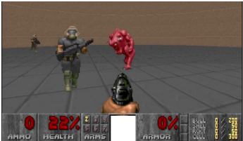
To understand why the last scenario (when τ ∗ > 0) is important, let us consider the example of the 3D FPS game Doom [Kempka et al., 2016]. Our initial failed attempt to learn a reward model for this game was the main inspiration behind the present work. In this challenging FPS task, an agent fights against two types of adversaries that have different dynamics and that appear randomly in a large open space around the agent. The agent gets a reward of +1 when it successfully shoots an adversary. It gets a reward of -1 when it dies. The agent does not have access to key information, such as the ammunition number and its health status. At each timestep, the agent can execute one of the following four actions: rotate left, rotate right, do nothing, and shoot. The agent then receives a reward and the position and dimensions of each object in the scene. To solve this task, the agent learns a reward function, and a transition function that maps each frame into a predicted next frame. The reward estimator is implemented as a neural network that takes as input current and a short history of object attributes (position and size) and a short history of executed actions. It outputs a probability distribution of possible rewards. A second neural network is used to predict future frames by forecasting changes in different attributes of objects. These two neural networks are trained from frames and rewards collected by using a random policy (i.e., uniform action distribution). After training, the learned networks are evaluated in test episodes with a lookahead tree search. At each time-step, the tree search simulates a large number of possible futures. Every branch of the search tree is obtained by recursively feeding the outputs of the transition network into itself and into the reward network, with different actions. The action with the highest predicted future rewards is then executed. The transition and reward networks also take as inputs the hidden memory units M discovered by the proposed algorithm. Details of the proposed transition and reward architectures are omitted due to lack of space.
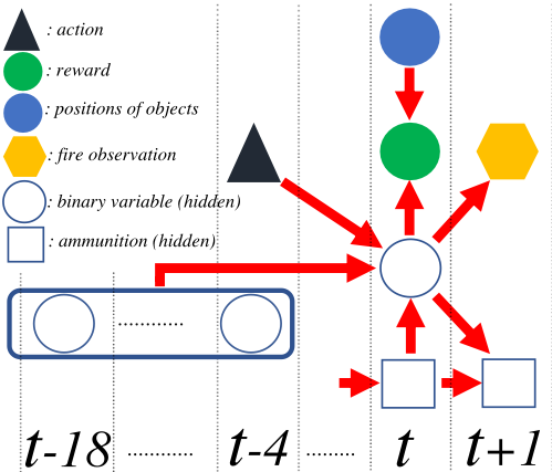
Surprisingly, predicting the reward for shooting was the most challenging part of this game. To receive a positive reward, the adversary should be exactly at the center of the image a few time-steps after the shooting takes place. Moreover, any shooting action that takes place less than 18 time-steps from a previous one is ineffective. The agent also runs out of ammunition after 26 rounds. Figure 1 shows the corresponding causality graph. The observed variables are: the executed action, the immediate reward, the positions and sizes of objects, and the appearance of a new object (fire) after every effective shooting. The remaining variables are hidden and unknown. Let Xt be the reward received at time t. Initially, the only parents of Xt are the executed action and the observed state of the objects at t - 1. To reduce the entropy of P(Xt|pa(Xt)), the algorithm searches for a variable Y that reduces the entropy of P(Xt|pa(Xt)) when it is included in pa(Xt). That variable turns out to be the appearance of fire at t + 1. If Xt → Yt+1 or Xt → Z → Yt+, then this information is useless when it comes to predicting Xt ahead of time. However, by applying the independence of input and mechanism test, the agent concludes that Xt is not a cause of Yt+1, and that we are rather in the case Z → Xt, Z → Yt+1. The algorithm then defers processing Xt to a later iteration, and proceeds into searching for past events that may cause Yt+1. This later observation cannot appear if the agent has not executed a shooting action at exactly t - 4, this past event is then automatically added to the parents of Yt+1 in the form of a hidden memory variable M1. The agent then also finds that the second most important variable for predicting Yt+1 is the elapsed time since the last appearance of fire, and adds a memory M2 of that event to the parents of Yt+1. The entropy of P(Yt+1|pa(Yt+1)) drops to almost zero with the inclusion of M1 and M2 in pa(Yt+1). Finally, reward Xt can be accurately predicted from the aggregated variable Z = (M1, M2) and objects' positions. This aggregated hidden variable Z is represented by the middle circle in Figure 1. It can be interpreted as a flag indicating if all the conditions for shooting are met. One may question why M1 and M2 were not directly added to the list of Xt's parents if they yield high information gain. The answer is that M1 and M2 do not yield noticeable information gains for Xt when taken individually, because reward Xt is sensitive to other attributes such as positions and sizes of objects which are high-dimensional, and instances of positive rewards Xt = +1 are rare in the data generated by a random exploratory policy. The observation of fire at the next step, denoted by Yt+1, is a deterministic outcome of M1 and M2. Thus, M1 and M2 are more easily detected as parents of Yt+1. Since all new parents of a variable are concatenated into a single variable (line 25), (M1,M2) will be selected in line 9 when Xt is processed again. This structure was automatically discovered by Algorithm 1. The algorithm failed, however, to discover the causal relation between ammunition (another hidden variable) and effectiveness of shooting actions. But this did not impact the performance of the planned policy, as we will see in the next section.
5 Experiments
The proposed approach is evaluated on three tasks. The first two are robotic experiments using the Gazebo simulator, and the third one is from the 3D FPS game Doom. The policy obtained from the learned transition and reward models for painting is evaluated using the real Kuka robot. The proposed method is compared with the model-free RL algorithms PPO and A2C, and the model-based RL techniques of [Oh et al., 2015] and [Chiappa et al., 2017]. All these methods use LSTM units. We also compare against a version of [Oh et al., 2015] that uses a GRU instead of an LSTM, and the method of [Vaswani et al., 2017] that uses an attention mechanism. We finally compare against a variant of our method that uses the same dynamics and reward architectures, but without including the memory variables.
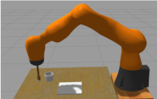
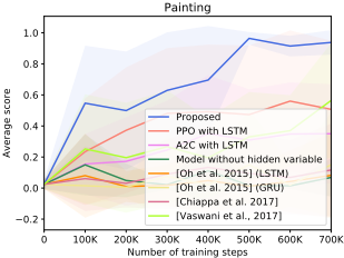
Painting. We formulate the painting problem illustrated in Figure 2 as a POMDP, where the state space corresponds to the position of the paintbrush attached to the robot's endeffector, and a hidden binary variable that indicates if the paintbrush is loaded. It is important to note that the robot observes only the position of the brush, and not if it is loaded or unloaded. The action space corresponds to movements of the end-effector in six directions. We use the Gazebo simulator with the MoveIt! path planner to move the end-effector between two adjacent cells and generate data. The length of each episode is 100 time-steps. When the brush goes inside the paint bucket, the binary variable switches from false to true and remains so until the end of the episode. This simple transition is difficult to learn because the binary switch variable can never be observed, there is no immediate evidence related to it, and the robot is even unaware of its existence a priori. If the paintbrush was loaded, the robot receives a reward of +1 when the brush touches the canvas. In all other cases, the received reward is 0. The reward function is also unknown and needs to be learned from the observed trajectories. Given that the data is collected with a random policy, the time difference between dipping the brush into the bucket and touching the canvas can be arbitrarily long. Using the proposed algorithm, the robot learned a state transition model and a reward function from data. The learned model was then used to return a policy. Results reported in Figure 3 show that our algorithm converges to a nearly 100% success rate. The Tire Changing Proposed PPO with LSTM
A2C with LSTM
Model without hidden variable
[Oh et al. 2015] (LSTM)
[Oh et al. 2015] (GRU)
[Chiappa et al. 2017]
[Vaswani et al., 2017]
0
25K
50K
75K
100k 125k
150k
Number of training steps Vizdoom - defend the center Proposed PPO with LSTM
A2C with LSTM
Stacking History
[Oh et al. 2015] (LSTM)
[Oh et al. 2015] (GRU)
[Chiappa et al. 2017]
[Vaswani et al., 2017]
0 100K 200K 300K 400K 500K 600K 700K 800K 900K 1M
Number of training steps
Figure 3: Average reward per test episode as a function of the number of time-steps in the training data. Stacking History refers to a variant of our architecture where the hidden variables are replaced with a long history of actions, observations and rewards.
results are averaged over 200 test episodes and five different initial positions of the paint bucket and the canvas.
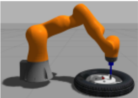
Tire Removal. The painting experiments involve only one hidden variable. To test the proposed algorithm on problems with more variables, we designed a second task in Gazebo where the robot is tasked with removing a tire. We assume that the robot is already equipped with an automatic drill on its end-effector, and the task consists in placing the drill on the lug nuts to loosen them before moving to the center of the wheel to take it off. The problem is formulated in the same way as in the painting task, except that the hidden variables now correspond to the status of each of four lug nut (tight vs. loose). The wheel can be taken off only when the endeffector is placed at the center of the wheel, after placing it on four specific points corresponding to the lug nuts. A reward of 1 is given when the task is successfully finished, all other states have a reward of 0. Results in Figure 3 and Table 1 confirm that the proposed approach discovers the causal link between visiting four specific regions of the state space and receiving a positive reward at the end of the episode. Note that the positions of the nut lugs are randomly selected at the beginning of each episode.
DoomGame. This task is presented in the example section. The transition and reward networks take as inputs the hidden memory variables M discovered by the proposed algorithm, in addition to the observations. The memory variables played a major role in speeding up the learning process. In Figure 3, we compare against a version of our architecture (denoted as stacking history) that replaces the hidden variable inputs with a long history of actions and observations. Here again, the proposed method significantly outperformed all the compared methods in terms of average score per episode.
| Task | Proposed | LSTM | GRU | Chi * | Vas † |
|---|---|---|---|---|---|
| Painting Reward 0 | 1/0.99 | 1/0.99 | 1/0.99 | 1/0.99 | 0.99/0.99 |
| Painting Reward 1 | 0.93/1 | 0/0 | 0/0 | 0/0 | 0.08/0.152 |
| Tire Reward 0 | 1/0.99 | 1/0.99 | 1/0.99 | 1/0.99 | 1/0.99 |
| Tire Reward 1 | 0.93/1 | 0/0 | 0/0 | 0/0 | 0/0 |
| VizDoomReward 0 | 0.99/0.99 | 1/0.99 | 1/0.99 | 1/0.99 | 1/0.99 |
| VizDoomReward 1 | 0.87/0.86 | 0/0 | 0.01/0.20 | 0/0 | 0/0 |
Final remark. A video of the robot experiments and more technical details are included in the project's page, https:// tinyurl.com/buxrmk4n .
Acknowledgments
This work is supported by NSF awards IIS-1734492 and IIS1846043.
@inproceedings{ijcai2021p268,
  title     = {Inferring Time-delayed Causal Relations in POMDPs from the Principle of Independence of Cause and Mechanism},
  author    = {Liang, Junchi and Boularias, Abdeslam},
  booktitle = {Proceedings of the Thirtieth International Joint Conference on
               Artificial Intelligence, {IJCAI-21}},
  publisher = {International Joint Conferences on Artificial Intelligence Organization},
  editor    = {Zhi-Hua Zhou},
  pages     = {1944--1950},
  year      = {2021},
  month     = {8},
  note      = {Main Track},
  doi       = {10.24963/ijcai.2021/268},
  url       = {https://doi.org/10.24963/ijcai.2021/268},
}
TY - CPAPER TI - Inferring Time-delayed Causal Relations in POMDPs from the Principle of Independence of Cause and Mechanism AU - Liang, Junchi AU - Boularias, Abdeslam T2 - Proceedings of the Thirtieth International Joint Conference on Artificial Intelligence, IJCAI-21 PB - International Joint Conferences on Artificial Intelligence Organization PY - 2021 SP - 1944 EP - 1950 DO - 10.24963/ijcai.2021/268 UR - https://doi.org/10.24963/ijcai.2021/268 ER -Copied
Machine-readable versions of this paper, for tools and AI agents:





