Reasoning about Beliefs and Meta-Beliefs by Regression in an Expressive Probabilistic Action Logic

1 Introduction

Because of its expressiveness, first-order logic (FOL) has played a key role in knowledge representation and reasoning since the beginnings of AI [McCarthy, 1963]. Since uncertainty is ubiquitous in many domains like robotics, it seems natural to combine FOL and uncertainty, mixing both categorical beliefs and degrees of belief. Such formalisms are especially useful when reasoning about the beliefs of robots acting and perceiving in uncertain environments.

In a seminal paper, Bacchus, Halpern, and Levesque (BHL) [1999] gave a very rich account of dealing with stochastic actions and noisy sensing as an extension of Reiter's version of the situation calculus [Raymond, 2001]. A key advantage of BHL's account is that it allows partial specifications of (subjective) beliefs, depending on what information is actually available in a particular domain.

∗Contact Author

Belle and Lakemeyer (BL) [2017] proposed an alternative formulation of BHL's ideas based on a modal variant of the situation calculus [Lakemeyer and Levesque, 2004], extending earlier work on static probabilistic beliefs [Belle et al., 2016]. In contrast to BHL, which is purely axiomatic, BL's logic DS comes equipped with a possible-world semantics together with distributions over worlds. Here a distribution is defined in terms of an assignment of non-negative numbers to the possible worlds. An epistemic state is modeled as a set of distributions and a sentence φ is believed with degree r initially, roughly, if for each distribution in the epistemic state the sum of the normalized weights of the worlds that satisfy φ is r. Beliefs after performing a sequence of actions are then defined using the notions of action likelihood and observational indistinguishability, which captures the idea that an agent may not be able to distinguish between certain actions.

The logic has a number of interesting properties such as full introspection of beliefs. It also comes equipped with a notion of only-believing to capture the beliefs of a knowledge base (KB) consisting of a set of sentences with degrees of belief attached to them. Despite its appeal DS also has shortcomings. Perhaps the main one is the lack of expressiveness when it comes to degrees of belief. Currently, the language allows to express degrees of belief only as constants or, more precisely, standard names representing rational numbers. However, it is clearly desirable to express that an agent believes that the values of a random variable are, say, geometrically distributed. 1 Likewise, while an epistemic state in DS consists of a set of distributions, which in principle would allow an agent to have incomplete information about what distribution is the correct one, this can also not be expressed. Considering a running example drawn from from BL (Figure 1), BL allows a formula like B(h = 3: .5) ∧B(h = 4: .5) to express that the robot believes the distance h to the wall is 3 or 4 with equal degree, yet a geometric distribution with expectation 2, like ∀u.B(h = u: G(u, 12 )), is not expressible in BL. Similarly, it may be desirable to express that all the agent believes is that the distribution of the distance to the wall is geometric with expectation unknown.

1 Since the domain of DS is countable, only discrete distributions are considered.

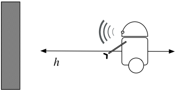
Another peculiar aspect of DS is that the beliefs of an agent depend on properties of the actual world, that is, changing the world can affect an agent's beliefs even though no (sensing) actions have occurred.

Finally, besides these issues, another important missing piece in BL's work is the lack of consideration of how to perform projection, that is, reasoning about future beliefs in a dynamic setting.

In this paper, we will address these shortcomings by extending the language and modifying the semantics of DS. In particular, this allows us to characterize probabilistic KBs (using only-believing), where an agent has incomplete information about belief distributions. Our main technical result is a solution to the projection problem by a novel form of regression. While regression under uncertainty has been considered in the past, we show, for the first time, how to deal with nested beliefs and quantifying into beliefs (quantifying-in).

The rest of the paper is organized as follows. In Section 2, we introduce the syntax and semantics of the new logic called DS ∗ . In Section 3, we investigate the properties of the logic. Regression is presented in Section 4. Finally, we discuss related work in Section 5 and conclude.

2 The Logic DS ∗

2.1 Syntax

DS ∗ is a first-order modal language with equality and sorts of type object and action. Implicitly, we assume that number is a sub-sort of object and refers to the computable numbers C. 2 Logical symbols include the usual symbols {=, ∧, ∀, ¬} and abbreviations {∃,≡,⊃}, as well as variables of every sort. There are function symbols of every sort and arity:

fluent function symbols of every arity, such as distance(x), nextTo(x,y), including two unary special symbols poss, l and a special binary symbol oi. Roughly, poss specifies when an action is possible (preconditions), l returns the likelihood of an action and oi describes the observational indistinguishability (alternative choices) among actions;

rigid function symbols of every arity, such as sonar(x), including arithmetical functions like +, -, ×, etc.

While fluent functions may vary due to actions, rigid functions are fixed. For simplicity, all action functions are rigid and we do not include predicate symbols in the language.

2 We use the computable numbers as they are still enumerable and allow representing distributions mentioning certain real numbers such as Euler's number e.

The language features a countable set of so-called standard names N, which are isomorphic with a fixed universe of discourse. Roughly speaking, this amounts to having an infinite domain closure axiom together with the unique name assumption. N = NO ∪ NA where NO and NA are object standard names and action standard names respectively.

The set of terms is the least set which contains the standard names N , variables of sort object (u, v, x, y, . . .) and action (a, a′ , . . .), and if t1, . . . tk are terms, f a k-ary function symbol, then f(t1, . . . tk) is in the set.

Ground terms are terms without variables. Primitive terms are terms of the form f(n1, . . . nk), where f is a function symbol and ni are object standard names. We denote the sets of primitive terms of sort object and action as PO and PA, respectively. While object standard names are syntactically like constants, we require that action standard names are all the primitive action terms, i.e. NA = PA. For example, the action sonar(5), where a sonar returns the number 5, is considered a standard action name. For any action term A(t1, . . . tk), A is referred to as the action type. 3 Furthermore Z refers to the set of all finite sequences of action standard names, including the empty sequence 〈〉. We reserve standard names ⊤, ⊥ in NO for truth values (to simulate predicates).

The set of formulas is the least set which contains atoms, (t = t′ ) where t and t′ are terms, and if α and β are formulas, x is a variable, r, ri are rigid terms (terms without fluent functions) of sort number, ta is of sort action, then ¬α, α∧β, ∀x.α, [ta]α, □α, B(α: r) and O(α1 : r1, . . . , αk : rk) are in the set.

[ta]α should be read as "α holds after action ta" and □α as "α holds after any sequence of actions." The epistemic expression B(α: r) should be read as "α is believed with probability r". Kα means "α is known" and is an abbreviation for B(α: 1). O(α1 : r1, . . . αk : rk) may be read as "the αi with a probability ri are all that is believed". Similarly, Oα means "α is only known" and is an abbreviation for O(α: 1). For action sequence z = a1 · · · ak, we write [z]α to mean [a1] · · · [ak]α. αx t is the formula obtained by substituting all free occurrences of x in α by t.

A sentence is a formula without free variables. We use TRUE as an abbreviation for ∀x(x = x), and FALSE for its negation. A formula with no □ is called bounded; a formula with no □ or [ta] is called static; a formula with no B or O is called objective; a formula with no fluent, □ or [ta] outside B or O is called subjective; a formula with no B, O, □, [ta], poss, l, oi is called a fluent formula; a fluent formula without fluent functions is called a rigid formula.

2.2 Semantics

The semantics is given in terms of possible worlds, which define what is true initially and after any sequence of actions. Compared to non-probabilistic accounts with deterministic actions [Lakemeyer and Levesque, 2004], a number of challenges need to be addressed, including how to specify probabilities over uncountably many possible worlds, how to deal with multiple probability distributions entertained by the agent, and how to deal with probabilistic action effects, which may be unobservable by the agent.

3 An action type is a set of actions that have the same action symbol but bound to different parameters, e.g. sonar(1), sonar(2) are of the same action type

A world w is a mapping from the primitive terms (PO ∪ PA) and Z to N of the right sort, satisfying:

1. Rigidity: If t is a rigid primitive term, then for all (w, z), (w′ , z′ ), w[t, z] = w′ [t, z′ ];
2. Arithmetical Correctness: If f is an arithmetical expression and val is its value in the usual sense, then for all (w, z), w[f, z] = val. For example, w[1 + 1, z] = 2.

We will sometimes also use piecewise rigid functions such as f(x) = .3 if x ∈ {3, 4, 5} and 0 o.w. We assume that these are simply built into the logic as well. 4

Let W be the set of all such worlds. Free variables are handled substitutionally by using standard names. We now define the notion of co-referring standard name for ground terms. Given a ground term t, a world w, and action sequence z, we define |t|zw (read: the co-referring standard name for t given w, z) recursively by :

1. If t ∈ N, then |t|zw = t;

For a rigid term t, we use |t| instead of |t|zw for its denotation. We will require that l(a) is of sort number, poss(a) and oi(a, a′ ) only take values ⊤ or ⊥, and oi behaves like an equivalence relation (reflexive, symmetric, and transitive). oi(a, a′ ) means a and a′ are observationally indistinguishable actions. In the example of Fig. 1, the robot might perform a stochastic action fwd(x, y), where x is its intended forward distance and y is the actual outcome selected by nature. x is observable to the robot while y is not. Then, oi(fwd(1, 1.1), fwd(1, 0.9)) says that nature can nondeterministically select 1.1 or 0.9 as a result for the intended value 1.

By a distribution d we mean a mapping from W to C≥0 (non-negative computable numbers) and an epistemic state e is any set of distributions. By a model, we mean a triple (e, w, z). In order to prepare for the semantics, we need to extend l(a), oi(a, a′ ), poss(a) from actions to action sequences:

Definition 1. We define

1. exec(z) as

Obviously, ∼w is an equivalence relation. Since W is uncountable, to obtain a well-defined sum over uncountably many worlds, the following three conditions are used for evaluating beliefs below:

4 Alternatively, one could add them as additional assumptions whenever needed.

Definition 2. We define BND, EQ, NORM for any distribution d and any set V = {(w1, z1), (w2, z2), . . .} as follows:

1. BND(d, V, n) iff ¬∃k, (w1, z1), . . . , (wk, zk) ∈ V such that ∑ki=1 d(wi) × l∗ (wi, zi) > n.
2. EQ(d, V, n) iff BND(d, V, n) and there is no n′ < n such that BND(d, V, n′ ) holds.
3. for any U ⊆ V, NORM(d, U, V, n) iff ∃b ̸= 0 such that EQ(d, U, b × n) and EQ(d, V, b).

Intuitively, given NORM(d, U, V, n), n can be viewed as the normalized sum of the weights of worlds in U wrt d in relation to V. Here EQ(d, V, b) expresses that the weight of the worlds wrt d in V is b, and finally BND(d, V, b) ensures the weights of worlds in V is bounded by b. In essence, even if W is uncountable, the condition EQ and BND admit a welldefined summation of the weights on worlds. See [Belle et al., 2016] for a formal justification of this claim.

The truth of sentences in DS ∗ is defined as:

• e,w, z |= t1 = t2 iff |t1|zw and |t2|zw are identical;
• e, w, z, |= ¬α iff e, w, z ̸|= α;
• e,w, z |= α∧ β iff e,w, z |= α and e,w, z |= β;
• e, w, z |= ∀x.α iff e, w, z |= αxn for every standard name n of the right sort;
• e, w, z |= [ta]α iff e, w, z · n |= α and n = |ta|zw ;
• e,w, z |= □α iff e,w, z · z′ |= α for all z′ ∈ Z.

To prepare for the semantics of epistemic operators, let We,z α = {(w′ , z′ ) | z′ ∼w′ z, and e,w′ , 〈〉 |= [z′ ]α ∧ exec(z′ )}. If z = 〈〉, we write Weα and if the context is clear, we write Wα. Intuitively, Wα is the set of alternatives (world and action sequence pairs) of z that might result in α.

Finally, after actions, we will restrict ourselves to compatible epistemic states that agree on action likelihood:

Definition 3. A distribution d is compatible with action sequence z, d ∼comp z iff NORM(d,W{d},z TRUE , W{d},z TRUE , 1); A distribution d is regular iff d ∼comp 〈〉.

Essentially, there are two cases where a distribution d may be incompatible with an action sequence z. First, EQ(d, W {d},z TRUE , 0), i.e. z has zero-likelihood in d. Second, ¬BND(d, W {d},z TRUE , r) for all r. This may happen, for example, if d assigns equal weights to all worlds in W. Distributions of this sort are called unmeasurable [Belle et al., 2016]. Regular distributions are just the measurable ones.

Let (e, w, z) be a model and ez = {d|d ∈ e, d ∼comp z}. We are now ready to define the semantics of B and O:

• e,w, z |=B(α: r) iff ∀d ∈ ez, NORM(d,W{d},z α ,W{d},z TRUE , n) and n = |r|;
• e,w, z |= O(α1 : r1, . . . , αk : rk) iff ∀d, d ∈ ez iff NORM(d, W{d},z αi , W{d},z TRUE , ni) for all 1 ≤ i ≤ k where ni = |ri| .

For any sentence α, we write e, w |= α instead of e, w, 〈〉 |= α. When Σ is a set of sentences and α is a sentence, we write Σ |= α (read: Σ logically entails α) to mean that for every set of regular distributions e and w, if e,w |= α′ for every

α′ ∈ Σ, then e,w |= α. We say that α is valid (|= α) if {} |= α. Satisfiability is then defined in the usual way. If α is an objective formula, we write w |= α instead of e,w |= α. Similarly, we write e |= α instead of e,w |= α if α is subjective.

2.3 Comparison with DS

The language of DS differs slightly from DS ∗ in that DS considers fluent predicates instead of fluent functions. Moreover, while in DS every closed term is a standard name, we follow [Lakemeyer and Levesque, 2011], who use special standard names for objects and actions. The semantic structures in both logics are essentially the same, consisting of worlds, sets of distributions over worlds serving as epistemic states, and action sequences. Our use of rigid mathematical functions, which are not considered in DS, is similar to the R-interpretation in [Belle and Levesque, 2018].

Since the semantic rules for B and O in both logics are similar, but differ in important details, it is instructive to review their definitions in DS. The main difference lies in how Wα is defined and used. DS uses the notion of compatibility between worlds: w′ ≈oi w iff for all a, a′ and z, w′ [oi(a, a′ ), z] = w[oi(a, a′ ), z], that is, w′ is compatible with w if they agree on the values of oi. Wα in DS is then defined wrt. triples e,w, z: We,w,z α = {(w′ , z′ ) | z′ ∼w′ z,w′ ≈oi w, and e,w′ , 〈〉 |= [z′ ]α ∧ exec(z′ )}. Note that worlds in We,w,z α agree with w wrt. observational indistinguishability. Belief is then defined as e,w, z |=DS B(α: n) iff ∀d ∈ e (not ez) , NORM(We,w,z α ,WTRUE, n) for constant n (and similarly for O).

The first thing to note is that our semantics of B (and O) is independent of the real word, while DS is not. In particular, the truth of B(α: n) depends on both e and w because of the definition of We,w,z α . As a result, even if e is kept fixed, once w changes, beliefs can vary. For example, consider a fluent lightOn, which indicates whether a light is on or off. In DS, using functions as in DS ∗ instead of predicates, we obtain:

Example 1. Let Σoi be □oi(a, a′ ) = ⊤ ≡ lightOn = ⊥ ∨ lightOn = ⊤ ∧ a = a′ . 5 Let w, w′ be two worlds such that w |=DS lightOn = ⊤ and w′ |=DS lightOn = ⊥. Additionally, suppose e,w |=DS KΣoi and e,w′ |=DS KΣoi. Then it follows that e,w |=DS K(lightOn = ⊤) and e,w′ |=DS K(lightOn = ⊥).

In English: Σoi says actions are mutually distinguishable if the light is on. There are two worlds w,w′ where the light is on and off, respectively. The agent with epistemic state e knows Σoi in both worlds. Then it follows that in world w the agent knows that the light is on while in w′ the agent knows that the light is off. This seems counter-intuitive, especially since the agent has not performed any actions.

This is the main reason why in DS ∗ the definition of Wα does not refer to the real world. We remark for the same reason we require the r in B(α : r) to be rigid and hence worldindependent (and similarly for O). But note that r can otherwise be an arbitrary mathematical function, allowing us to express things like distributions as in ∀u.B(h = u: G(u, 1 2 )).

5 Free variables are implicitly universal quantified outside. The modality □ has lower syntactic precedence than the connectives, and

[·] has the highest priority.

Lastly, notice that in the definition of B and O, we use W{d},z α instead of We,z α (or We,w,z α as in DS ∗ ). While this makes no difference when it comes to believing objective sentences, it does impact beliefs about beliefs in important ways, in particular introspection, as discussed below. Perhaps the greatest benefit of this change is that only-believing a sentence becomes uniquely satisfiable in DS ∗ . Among other things, this allows us to model agents which are unsure about their beliefs. For example, if p is an atomic sentence, then O(B(p : .3) ∨B(p : .4)) is satisfied by the set of all regular distributions where the degree of belief in p is either .3 or .4. Yet, in DS the above sentence is unsatisfiable.

3 Properties of Belief and Only-believing

The new logic shares many properties with DS like additivity, and the Barcan formula. Formally, we have:

Proposition 1. for any formula α, β and rigid terms r, r′ , r′′ :

1. If |= □(α = β) then |= (B(α: r) ≡B(β : r));
2. |= □(B(α∧β : r) ∧B(α∧¬β : r′ ) ⊃B(α: r +r′ ));

1. |= □(Kα∧K(α ⊃ β) ⊃Kβ);
2. |= □(∀xKα ⊃K∀xα);
3. |= □(∃xKα ⊃K∃xα).

Introspection, which is valid in DS, is not valid in DS ∗ in general. However, as we will see below, it does hold under certain assumptions.

3.1 Introspection

In the static case, for positive introspection, we have:

Theorem 1. For any α and r, |=B(α: r) ⊃K(B(α: r)).

Negative introspection like ¬B(α: r) ⊃ K(¬B(α: r)) does not hold. For example, let {d1} |= B(α: r) and {d2} ⊭ B(α: r), then for e = {d1, d2}, we have e |= ¬B(α: r). Yet, e ⊭ K¬B(α: r) due to W{d1} ¬B(α: r) = ∅ and NORM(d1, W{d1} ¬B(α: r) ,W{d1} TRUE , 0).

Besides, □(B(α: r) ⊃ K(B(α: r)) is not valid in general. This is because we allow worlds with different observational indistinguishability in Wα, and as pointed out in DS, the consistency of observational indistinguishability between worlds and actions inWα (≈oi) are crucial for introspection. However, when oi is rigid, positive introspection holds.

where ψ is a rigid formula. Then we have:

Theorem 2. Let Σoi be as above. Then for any α and r, K(Σoi) |= □B(α: r) ⊃K(B(α: r))

Let us now consider a case where negative introspection also holds. By a belief distribution we mean the joint distribution of a finite set of random variables. Formally, assuming a finite set of nullary fluents ⃗h = {h1, . . . hm}, 6 a belief distribution Bf init of ⃗h is a formula of the form ∀⃗u.B(⃗h = ⃗u: f(⃗u)) , where ⃗u is a set of variables, ⃗h = ⃗u stands for ∧ hi = ui, f is a rigid function of sort number with free variables ⃗u. Taking our robot example, a belief distribution might be Bf init (for the single fluent h), where f is given by

Such belief distributions will play an important role later.

Lemma 1. Let Bf init be a joint belief distribution and α a subjective static formula whose fluents are all in Bf init , then Bf init |= α or Bf init |= ¬α.

The proof is by induction on the size of formula α. The lemma says, roughly, that Bf init determines completely what the agent believes and does not believe.

Theorem3. For any α, r, let Bf init be a belief distribution of fluents in α and Σoi as before:

• Bf init |= ¬B(α: r) ⊃K(¬B(α: r));
• Bf init ∧K(Σoi) |= □¬B(α: r) ⊃K(¬B(α: r)).

The first part holds as a direct consequence of Lemma 1: once an epistemic state satisfies Bf init and ¬B(α: r), then all distributions considered must satisfy ¬B(α: r), hence K(¬B(α: r)) is satisfied. The proof of the second is rather similar to its counter-part of the positive introspection.

3.2 Only-believing

Let us now turn to the notion of only-believing, which is intended to capture the beliefs of an agent's probabilistic KB.

Proposition 2. Let αi be arbitrary sentences and ri arbitrary rigid terms of sort number, we have

1. |=O(α1 : r1; . . . αk : rk) ⊃ ∧ B(αi : ri);
2. |= O(α: r) ⊃ ¬B(h(⃗n) = m: r′ ) for all r, r′ , and α, where ⃗n and m are std. names and h is a fluent not in α;

The second part says that the agent has no beliefs about things not mentioned in the KB. Note that this is not true if O is replaced by B. The third part says only-believing reduces to only-believing a single subjective sentence with certainty.

Theorem 4 (Unique Model Theorem). For arbitrary αi and ri, there is a unique set of regular distributions e such that e |=O(α1 : r1; . . . αk : rk).

6 As discussed in [Belle and Levesque, 2018], allowing fluents with arguments would result in joint distribution over infinitely many random variables, which is generally problematic in probability theory.

Proof. Let e = {d | NORM(d,W{d} αi ,W{d} TRUE , ni), ni = |ri|, 1 ≤ i ≤ k}. Clearly e |= O(α1 : r1; . . . αk : rk), and there cannot be any other e with that property.

While only-believing is always uniquely satisfied by an e, it may be the case that e is empty. For example, ∅ |= O(p ∧ ¬p : .6) and ∅ |= O(O(p)). For the latter this is because no single distribution only-believes p.

We remark that in DS the unique-model property for O only holds for objective sentences. In the case of nonobjective sentences, there may be multiple epistemic states that only-believe them or none at all. For example and as mentioned earlier, O(B(p : .3)∨B(p : .4)) is not satisfiable in DS. Such feature makes DS ∗ much more expressive than DS and many other probabilistic formalism. For example, O(∃x.∀u.B(h = u: G(u, x))) says the agent only-believes that the distance is geometricly distributed.

4 Reasoning by Regression

An important reasoning task for the agent is to determine what holds after actions. Regression is a powerful technique to solve this problem by transforming a query about the future to a query about the initial state [Raymond, 2001]. In this section, we first introduce the notion of basic action theories (BATs) that are required for regression. Thereafter, we explore how regression works in the setting of beliefs.

4.1 Basic Action Theories

BATs were first introduced by Reiter [2001] to encode the effects and preconditions of actions. In a dynamic uncertain setting, BATs additionally have to specify the observational indistinguishability among actions and likelihoods of actions. Formally, given finite action types A1, . . .Ak, Σ = Σpre ∪ Σpost ∪Σoi ∪Σl consists of the union of these sets:

• Σpre: A set consisting of a single axiom of the form □poss(a) = ⊤ ≡ ∨i ∃⃗xi.a = Ai(⃗xi) ∧ πi to characterize action preconditions.
• Σpost: A set of successor state axioms, one for each fluent, of the form □[a]h = u ≡ ∨i ∃⃗ xi.a = Ai(⃗xi) ∧ γi ∨ ∧i ∀⃗ xi.a ̸= Ai(⃗xi) ∧ h = u to characterize action effects, also providing a solution to the frame problem [Raymond, 2001].
• Σl: A single axiom of the form□l(a) = q ≡∨i ∃⃗xi.a = Ai(⃗xi) ∧ φi to capture action likelihoods.

Here πi, γi, φi are fluent formulas with free variables among ⃗xi. γi (respectively, φi) has free variable u (q) and are functional in u (q). Moreover, Σoi consists of a single axiom as in Eq. 1, which forces oi to be rigid (Σoi is also in form of disjunctions wrt action types A1, . . . Ak).

Example 2. In our robot example, besides the stochastic action fwd(x, y), assume the robot can perform a noisy sensing sonar(z) to locate itself, where z denotes the observed value of sonar. Then the following is a possible BAT:

∨ a = sonar(z) ∧ q = θ(z, h, .2, .6), where

In English: actions are always executable; distance h can only be affected by fwd(x, y) and the value is determined by value y, not the intended value x; two actions are observationally indistinguishable if and only if they are both forward actions with the same intended value or they are identical sensing action; action likelihood is specified by θ.

4.2 Regressing Objective Formulas

The regression of objective formulas is similar to [Claßen, 2013]. A formula where each quantifier has a distinct variable is called rectified. Let TΣ be the set of action terms that can be generated by the finite action types of BAT Σ, i.e. TΣ = ∪i{Ai(⃗r)|⃗r are standard names or variables}. In the rest of the paper, action terms and action sequences refer to terms in TΣ and sequences in (TΣ)∗ .

An objective formula is called regressable if it is bounded, rectified and every function fluent has the form h = r′ , where r′ does not mention any fluent. In addition every poss and oi is of the form poss(t) = ⊤, oi(t, t′ ) = ⊤ s.t. t, t′ ∈ TΣ. 7 Apart from being bounded, all other syntactic restrictions on regressable formulas are only introduced for convenience in order to simplify the following definition. Unbounded formulas such as □α are not regressable because □ represents an infinite number of action sequences.

We define R[α], the regression of α wrt Σ, to be R[〈〉, α], with R[z, α] for any action sequence z ∈ (TΣ)∗ defined as:

• R[z, α] = α if α is rigid;
• R[z, ¬α] = ¬R[z, α], and similarly for ∧, ∀;
• R[z, [Ai(⃗r)]α] = R[z · Ai(⃗r), α];
• R[z, poss(Ai(⃗r)) = ⊤] = R[z, (πi)⃗xi ⃗r ], πi is from Σpre's RHS, and similarly for l and oi;
• R[z, h = r′ ] is defined inductively:

Note that R[α] always results in a fluent formula if α is regressable.

7 It is easy to see that every formula can be rewritten this way, e.g. |= h = h′ ≡ ∃x.h = x ∧ h′ = x, for fluents h, h′ .

Theorem 5 (Regression Theorem). Let D be a set of fluent sentences (describing the initial state), Σ a BAT, α a regressable sentence. Then D ∪ Σ |= α iff D |= R[α].

The proof follows the same argument as the proof a corresponding theorem in [Claßen, 2013]. As an illustration, consider the BAT Σ of the robot example. R[[fwd(1, 1)]h = 10] = (h = 9). So to determine whether [fwd(1, 1)]h = 10 is entailed by some D ∪ Σ, we only need to check whether D entails h = 9.

4.3 Regressing Beliefs

To reason about future beliefs, besides basic action theories, we need to specify what is believed initially. By the notion of a belief distribution, our initial KB is expressed via a single sentence of the form O(Bf init ∧ Σ), where Bf init is a belief distribution of fluents mentioned by BAT Σ.

The regression operator now takes a single belief distribution Bf init as a parameter, namely R[Bf init , z, α].

A formula is called regressable wrt Bf init if all fluents are mentioned in Bf init , it does not mention O, and otherwise satisfies the constraints for objective regressable formulas.

Taking the Bf init of the robot example (see Eq. 2), [fwd(1, 1)]K(h = 1) and [sonar(2)]K([fwd(1, 1)]B(h = 3: 12 )) are regressable, while □K(h = 1) and B(h = h′ : .6), are not, assuming h, h′ are fluents. If the context is clear, we leave out Bf init . Given a BAT Σ and z = t1 · t2 · . . . · tk where ti ∈ TΣ, if Bf init is compatible with z,Σ (Def. 4 below), the regression of belief is defined as:

where η is the normalizer, which has the same form as the numerator but replacing α with TRUE, ∑z′∈Ψ is an abbreviation of ∑t′1∈{t′′ 1 | |=ψ1} . . . ∑t′k ∈{t′′ k | |=ψk} , and ψi is the RHS of Σoi instantiated by ti and t′′ i . z′ = [t′1 ] . . . [t′k ]. ⃗u ranges over (NO)m where m is the number of fluents and t′i ranges over NA. 8

T[z, ⃗u] is recursively defined as:

= λ(R[z, l(t) = qt]⃗h ⃗u ) and λ is a function that extracts the value of qt after regression. Essentially LH(z, t, ⃗u) returns the likelihoods of action t after action sequence z, T[z, ⃗u] returns the likelihoods of z when the initial state satisfies ⃗h = ⃗u, and I(⃗u, α) indicates whether α follows from the initial state ⃗h = ⃗u. For space reasons, we leave out the details of how to specify λ, but the ideas are essentially the same as in [Belle and Levesque, 2020]. See the regression ex. below.

8 Note that summation is treated here like any other rigid mathematical function for simplicity. It can be defined using second-order logic as shown in [Belle and Levesque, 2018], for example.

Basically, f is compatible with z,Σ if and only if z has non-zero likelihood under f and Σ. In case Bf init is not compatible with z, Σ, we define: R[z, B(α : r)] ≡ TRUE

Theorem 6. Let D,Σ,Bf init be as before, then for all regressable formulas α,

The first equivalence is because Σoi declares an observational indistinguishability among fwd(x, y) for all y.

Note that LH(〈〉, fwd(1, y), u) = θ(1, y, .1, .8) and LH (fwd(1, y), sonar(3), u) = θ(3, u - y, .2, .6):

Therefore λ(∃u′ .u = u′ + y ∧ qt = θ(3, u′ , .2, .6)) = θ(3, u - y, .2, .6)). The second equivalence is because R[fwd(1, y), [sonar(3)]∃x. B(h = x: 58 )] (denoted as R[IN]) returns TRUE in the same vein as the outer regression:

Here, the second line holds because I(u, h - y′ = x) is nonzero only if u - y′ = x and θ(3, u - y′ , .2, .6) is non-zero only if u - y′ is among {2, 3, 4}. The third line is due to η′ = .32 by computation. Hence |= R[IN] and moreover |= R[fwd(1, 2),B(h = 2∧ [sonar(3)]∃x.B(h = x: 58 ): 3 10 )], By Theorem 6, O(Bf init ∧ Σ) |= [fwd(1, 2)]B(h = 2 ∧ [sonar(3)]∃x.B(h = x: 5 8 ): 3 10 ).

5 RelatedWork

Our logic builds on DS [Vaishak and Gerhard, 2017], a modal logic of degrees of belief based on a modal variant of the situation calculus [Lakemeyer and Levesque, 2011]. In particular, our logic allows to express belief distributions, while the degree of belief in DS is restricted to numbers. BHL define Bel via a special fluent p and belief distributions can be expressed axiomatically, but they leave the question of how to represent an agent's KB open.

The concept of only-believing to capture the beliefs of a KB was first introduced by Levesque [1990], from which the version in DS derives. Only-believing without full introspection was studied in [Humberstone, 1987].

Reasoning about knowledge and probability has been addressed in many domains: in computer science [Nilsson, 1986; Fagin and Halpern, 1994] , in game theory [Monderer and Samet, 1989; Aviad and Philippe, 2001] among others [Halpern, 2003]. The work of [Fagin and Halpern, 1994] is at the heart of BHL and this work. Most recently, [Belle and Levesque, 2018] reconsiders the BHL framework and extends it to continuous domains.

In terms of belief regression, our ideas are inspired by [Belle and Levesque, 2014b], an extension of [Belle and Levesque, 2013a; Belle and Levesque, 2013b] where regression is proposed for the BHL framework. What distinguishes us perhaps most is that our regression operator works for meta-beliefs as well.

The main challenge of regression in stochastic domains is how to address noisy sensor and effectors. This has been studied in standard probabilistic frameworks [Fox et al., 2003; Thrun et al., 2005; Boyen and Koller, 1998], and in symbolic programming [Boutilier et al., 2001; Boutilier et al., 2000].

6 Conclusions

We proposed a logic of belief for the specification of very expressive KBs in uncertain dynamic domains. Our main result is a novel form of regression which applies to beliefs about beliefs, including quantifying-in. We remark that, while our result assumes a single initial belief distribution, we believe that it can be extended to multiple distributions.

For future work, projection by progression, that is, by modifying the initial beliefs, is an interesting avenue. Existing work on progression like [Belle and Lakemeyer, 2011; Belle and Levesque, 2014a] may be a good starting point. Another direction would be to use the logic for the verification of belief programs [Belle and Levesque, 2015].

Acknowledgments

This work has been supported by the Deutsche Forschungsgemeinschaft (DFG, German Research Foundation) RTG 2236 'UnRAVeL' and by the EU ICT-48 2020 project TAILOR (No. 952215).