
Compressing Exact Cover Problems with Zero-suppressed Binary Decision Diagrams
Proceedings of the Thirtieth International Joint Conference on Artificial Intelligence. Main Track. Pages 1996-2004.
https://doi.org/10.24963/ijcai.2021/275
Keywords
- Knowledge Representation and Reasoning: Knowledge Representation Languages
- Heuristic Search and Game Playing: Combinatorial Search and Optimisation
Abstract
Exact cover refers to the problem of finding subfamily
F of a given family of sets S whose universe
is D, where F forms a partition of D. Knuth’s Algorithm
DLX is a state-of-the-art method for solving
exact cover problems. Since DLX’s running
time depends on the cardinality of input S, it can be
slow if S is large. Our proposal can improve DLX
by exploiting a novel data structure, DanceDD,
which extends the zero-suppressed binary decision
diagram (ZDD) by adding links to enable efficient
modifications of the data structure. With DanceDD,
we can represent S in a compressed way and perform
search in linear time with the size of the structure
by using link operations. The experimental results
show that our method is an order of magnitude
faster when the problem is highly compressed.
- [Bryant, 1986] Randal E Bryant. Graph-based algorithms for boolean function manipulation. Computers, IEEE Trans. on, C-35(8):677-691, 1986.
- [Chabert and Solnon, 2020] Maxime Chabert and Christine Solnon. A global constraint for the exact cover problem: Application to conceptual clustering. Journal of Artificial Intelligence Research, 67:509-547, 2020.
- [Chang and Jiang, 2016] Hua-Yu Chang and Iris Hui-Ru Jiang. Multiple patterning layout decomposition consid- ering complex coloring rules. In DAC, 2016.
- [Choi et al., 2016] Arthur Choi, Nazgol Tavabi, and Adnan Darwiche. Structured features in naive Bayes classifica- tion. In AAAI, pages 3233-3240, 2016.
- [Cook and Seymour, 2003] William Cook and Paul Sey- mour. Tour merging via branch-decomposition. INFORMS J. on Computing, 15(3):233-248, 2003.
- [Coudert et al., 2014] David Coudert, Dorian Mazauric, and Nicolas Nisse. Experimental evaluation of a branch and error bound. Smart Grid, IEEE Trans. on, 5(1):102-111, 2014.
- [Junttila and Kaski, 2010] Tommi Junttila and Petteri Kaski. Exact cover via satisfiability: An empirical study. In CP, pages 297-304, 2010.
- [Karp, 1972] Richard M Karp. Reducibility among combi- natorial problems. In Complexity of computer computa- tions, pages 85-103. Springer, 1972.
- [Kawahara et al., 2017] Jun Kawahara, Takeru Inoue, Hi- roaki Iwashita, and Shin-ichi Minato. Frontier-based search for enumerating all constrained subgraphs with compressed representation. IEICE Trans. on Fundamen- tals of Electronics, Communications and Computer Sci- ences, E100.A:1773-1784, 09 2017.
- [Knight et al., 2011] Simon Knight, Hung X Nguyen, Nick- olas Falkner, Rhys Bowden, and Matthew Roughan. The internet topology zoo. IEEE Journal on Selected Areas in Communications, 29(9):1765-1775, 2011.
- [Knuth, 2000] Donald E Knuth. Dancing links. In Millenial Perspectives in Computer Science, pages 187-214, 2000.
- [Knuth, 2011] Donald E Knuth. The Art of Computer Pro- gramming, Volume 4A: Combinatorial Algorithms, Part 1. Addison-Wesley, 2011.
- [Knuth, 2019] Donald E Knuth. The Art of Computer Pro- gramming, Volume 4 Fascicle 5: Mathematical Prelim- inaries Redux; Introduction to Backtracking; Dancing Links. Addison-Wesley, 2019.
- [Koivisto, 2006] Mikko Koivisto. An O(2 n ) algorithm for graph coloring and other partitioning problems via inclusion-exclusion. In FOCS, pages 583-590, 2006.
- [Lagniez and Marquis, 2017] Jean-Marie Lagniez and Pierre Marquis. An improved decision-dnnf compiler. In IJCAI- 17, pages 667-673, 2017. IJCAI
- [Minato et al., 2008] Shin-ichi Minato, Takeaki Uno, and Hiroki Arimura. LCM over ZBDDs: Fast generation of very large-scale frequent itemsets using a compact graph- based representation. In PAKDD, pages 234-246, 2008.
- [Minato, 1993] Shinichi Minato. Zero-suppressed BDDs for set manipulation in combinatorial problems. In DAC, pages 272-277, 1993.
- [Nguyen et al., 2018] Vivian Nguyen, Bill Moran, Ana No- vak, Vicky Mak-Hau, Terry Caelli, Brendan Hill, and David Kirszenblat. Dancing links for optimal timetabling. Military Operations Research, 23(2):61-78, 2018.
- [Nishino et al., 2016] Masaaki Nishino, Norihito Yasuda, Shin-ichi Minato, and Masaaki Nagata. Zero-suppressed sentential decision diagrams. In AAAI, pages 1058-1066, 2016.
- [Nishino et al., 2017] Masaaki Nishino, Norihito Yasuda, Shin-ichi Minato, and Masaaki Nagata. Dancing with de- cision diagrams: A combined approach to exact cover. In AAAI, pages 868-874, 2017.
- [Suzuki and Minato, 2016] Hirofumi Suzuki and Shin-ichi Minato. Adding the vertex indices for enumerating and indexing the graphs via zdd (in japanese). Special Interest Group on Fundamental Problems in Artificial Intelligence, 101:41-46, 2016.
- [Thurley, 2006] Marc Thurley. sharpSAT -counting models with advanced component caching and implicit BCP. In SAT, pages 424-429, 2006.
References were extracted automatically from the PDF and may contain errors.
Full text extracted automatically from the PDF; figures, tables and equations may differ. The PDF is the version of record.
1 Introduction
An exact cover refers to the problem of finding subfamily F of a given family of sets S whose universe is D, where F forms a partition of D; that is, ⋃X∈F X = D and X ∩X′ = ∅ for all X ̸= X′ ∈ F. A wide range of problems, including puzzles like N-queens [Knuth, 2000], Sudoku [Gunther and Moon, 2012], and graph coloring [Koivisto, 2006], can be formulated as exact cover problems. Determining whether a solution exists for an exact cover problem is known to be NP-complete [Karp, 1972].
Knuth's Algorithm DLX (DLX) [Knuth, 2000] is a method for solving an exact cover problem. DLX performs an exhaustive depth-first backtracking-based search by exploiting doubly linked list structures called dancing links. DLX is known as the state-of-the-art method for finding all solutions of an exact cover problem [Junttila and Kaski, 2010]. Enumerating solutions is beneficial if we consider exact covers appearing in practical situations, such as designing electric circuits [Chang and Jiang, 2016], designing 3D shapes from small fragments [Hu et al., 2014], and timetabling [Nguyen et al., 2018]. In such practical situations, users may want to compare multiple exact covers.
The space complexity of DLX is linear with the cardinality of S and a state transition in DLX requires time to be linear with it. Unfortunately, formulating a real-world problem as an exact cover problem often causes an exponential blowup of the cardinality of S. For example, the vehicle-routing problem finds a set of vehicle routes to reach and deliver all customers. This problem can be formulated as an exact cover problem. However, in such formulations, S corresponds to the set of all possible routes, which is generally exponential with the number of customers. In such cases, DLX would fail to find solutions to the exact cover problems.
In this paper, we propose a new algorithm, D3X, which is an extension of DLX, by exploiting a new data structure DanceDD to represent S in a succinct form. DanceDD is made by adding links to a zero-suppressed binary decision diagram (ZDD) [Minato, 1993], which can represent a family of sets in a compressed form. Algorithm D3X can perform the operations required for updating search states on a backtracking-based depth-first search in linear time to the ZDD size, which can be much faster than DLX when we can represent S as a compressed ZDD 1 .
2 AlgorithmDLX
We begin with a brief review of the exact cover problem and DLX. Let M be the cardinality of universe D = {1, . . . ,M} and N be the cardinality of S. Input S of an exact cover problem can be represented as a binary N ×M matrix A. Every row vector represents a set X ∈ S, where the i-th element of X is 1 iff i ∈ X and 0 otherwise. With this representation, an exact cover problem corresponds to finding a set of row vectors that contains exactly one 1 for each column. The matrix
represents an exact cover problem, where N = 5 and M = 6. In this example, the sets of options 2, 3 and 1, 3, 5 are the solutions. In the following, we call each X ∈ S an option and each j ∈ D an item.
DLX finds all solutions of an exact cover problem by performing a depth-first backtracking-based search. We show an overview of DLX in Alg. 1. Search(A, R) is the main procedure that recursively searches for solutions of the exact cover problem whose input is represented as binary matrix A, where R is a set of selected options representing the current partial solution. Search(A, R) first checks whether A has no remaining items (line 2). If the condition is true, it then outputs R as a solution and returns. Otherwise, it selects item i to cover (line 3). DLX uses the minimum remaining values (MRV) heuristic of selecting the item corresponding to a column with the minimum number of 1s in A. The MRV heuristic is simple, but works well in practice [Knuth, 2019]. The algorithm then selects the set of options O = {X | X ∈ A, i ∈ X} (line 4). It then chooses an option X from O and adds it to partial solution R (line 5). If option X is added in R, then no option X′ satisfying X ∩ X′ ̸= ∅ can be selected. We thus delete such options from A (line 9). The algorithm then recursively calls Search(A, R) to continue the search. After the search has finished, it restores all options and items that are deleted after selecting X (lines 12 and 13) and then selects another option from O to repeat the procedure.
1 Our code is available at https://github.com/nttcslab-alg/d3x
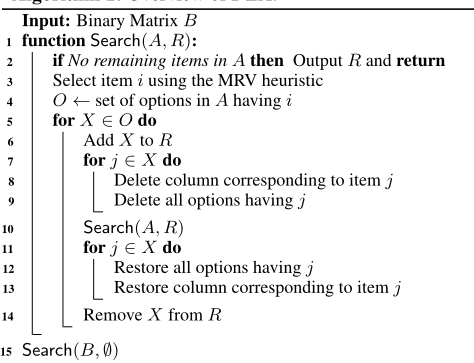
Example 1. Suppose that the matrix shown in (1) is given as the input of DLX. DLX first calls Search(A, ∅). In this example, the MRV heuristic would select an item from a, b, d, e, f . Suppose that item a is selected at line 3. Then, the set of options (row vectors) having item a is O = {{a, b}, {a, b, c, e}}. When the algorithm selects the first option {a, b} and adds it to R, items a and b, and options having either a and b, are then deleted (lines 7-9). The following submatrix is obtained by deleting them:
We recursively call Search(A, R) by setting the submatrix as A and R = {{a, b}}. In the recursive call, the MRV heuristic selects item e and appends the fifth option {c, e} to R since it only contains e. Thus, items c and e, and options 4 and 5, are deleted, which yields submatrix
Next, selecting the third option {d, f} covers all the items; thus, selected options 1, 5, 3 form an exact cover.
2.1 Dancing Links
Since DLX repeatedly deletes and recovers matrix elements, we need an appropriate data structure to run them efficiently. Dancing links is a data structure that enables efficient execution of these operations. Dancing links represents an input matrix by exploiting sets of doubly linked lists. Let x be a cell in a doubly linked list and let L(x) and R(x) be the previous and next cells to which the x points to. Using doubly linked lists, we can remove and recover elements from a list in constant time by using the following operations:
The former two operations remove x from the linked list and the latter restore it.
Dancing links represents an input matrix using two types of cells: item and node. An item cell corresponds to an item in universe D and has four links: left, right, up, and down. left and right indicate the previous and next item cells. We use a doubly linked list to represent the set of all item cells. The linked list has a special item cell header whose left and right links point to the first and last item cells. We say a cell is active if we can reach the cell from the header by following some links. down and up indicate the first and last node cells that correspond to item i. A node cell corresponds to an element of a binary matrix representing input S. It has three links: up, down, and item. item points to the item cell to which the node cell corresponds, and up and down denote the previous and next node cells that have the same item field. An option is represented using an array of node cells where every node cell corresponds to an item in the option.
Figure 1(a) is a graphical representation of the dancing links structure. The rectangles in the top level represent the item cells and the blue squares represent the node cells. The top row denotes the set of items represented as a doubly linked list of item cells, where the arcs represent the left and right links. Other rows, which consist of node cells, represent options. The up and down links of the cells are also represented as arcs. The symbol in the rectangles represents the item to which the cell corresponds. We can see that the node cells in the figure correspond to the 1s of the binary matrix shown in (1).
DLX can delete and recover options by updating links. Here, we only show an example of how the structure changes during the search procedure. Interested readers can find details of DLX in [Knuth, 2000; Knuth, 2019]. Figure 1 (b) and (c) show the structure that appears after selecting option X = {a, b} in Example 1. Figure 1 (b) is obtained by deleting item a and options containing a. We can see that the item cells corresponding to a are removed from the linked list of item cells. Node cells appearing in options {a, b}, {a, b, c, e}
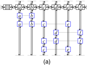
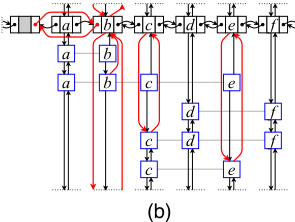
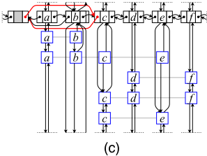
are also removed from linked lists connected by up and down links. Figure 1 (c) is obtained by further removing item b and options having b. The active node cells represent the submatrix in (2). We can perform these deletions using the link operations in (4). Its running time is linear with the number of cells to be removed. It is also possible to revert changes to recover the structure in Fig. 1 (a) from the structure in Fig. 1 (c) by exploiting the link operations (5), which also can be performed in linear time with the number of elements to be recovered.
3 ZDDs
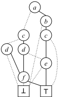
A ZDD represents a family of sets as a directed acyclic graph. Figure 2 is an example of a ZDD that represents the family of sets S = {{a, b},{a, b, c, e},{d, f},{c, d, f},{c, e}} over universe D = {a, b, c, d, e, f}. ZDDs have two types of nodes: terminal and branch. A terminal node has no outgoing edges. A ZDD has exactly two terminal nodes with labels ⊤ and ⊥. Terminal nodes are represented as rectangles in the figure. Branch nodes are non-terminal and are represented as circles in the figure. Every branch node has a label representing the item to which the node corresponds and two outgoing edges: low and high. ZDD nodes indicated by low and high edges of a branch node n are called the low-child and high-child of n, respectively. In the figure, a branch node's label is represented as a symbol in a circle, and high and low edges are represented by solid and dashed lines, respectively. A branch node without an ancestor node is the root node; a ZDD always has one root node. Every path from the root to the ⊤ terminal node corresponds to a subset X ∈ S. We can recover X from the corresponding path by selecting the labels of the branch nodes whose high edges lie on the path. The ZDD in Fig. 2 has five such paths and each path corresponds to a subset X ∈ S.
A ZDD is ordered if labels of visited branch nodes in a path from the root to a terminal node always follow an order over the universe. The ZDD in Fig. 2 is an ordered ZDD since every path from the root to a terminal node follows the order a, b, c, d, e, f. In the following, we assume that ZDDs are always ordered.
4 AlgorithmD3X
Our proposed D3X performs a backtracking-based depth-first search with the DanceDD structure representing input S. We first introduce the DanceDD structure (§4.1) and then show the search algorithm exploiting it (§4.2). We also compare the time and space complexity of D3X with DLX (§4.3).
4.1 The DanceDD Structure
Since input S of an exact cover problem is a family of sets, it can be represented in a compressed form by using ZDD. Figure 2 is a ZDD representing the set family corresponding to binary matrix (1). In this example, the number of ZDD branch nodes is 8, which is less than 13, which is the number of nonzero elements of the matrix. Although the size of the ZDD depends on the target being represented, it is known that the number of branch nodes of a ZDD is always not larger than the number of 1s in the binary matrix representing S [Minato et al., 2008].
DanceDD is made by adding links to an input ZDD. The dancing links structure used in DLX enables the deletion and restoration of matrix elements by modifying links. Similarly, DanceDD can delete and restore ZDD branch nodes by modifying links. It enables running an efficient depth-first search on a compressed representation. Similar to the dancing links structure, DanceDD consists of two types of cells: item and node. An item cell is identical to that used in the dancing links structure, which has four links, left, right, up, and down, and one non-negative integer field, len. A node cell corresponds to a ZDD branch node and has seven links: up, down, item, lo, hi, head, and tail. up and down indicate the next and previous cells that correspond to the same item and item indicates the corresponding item cell in the header. lo and hi point to the node cells corresponding to the low- and high-child ZDD nodes. head and tail are used to store the addresses of node cells corresponding to parent
Algorithm 2: Algorithm D3X
1 function SearchZDD(R): 2 if A is empty then Output R and return 3 Select item i using the MRV heuristic. 4 CoverZDD(i) 5 p ← down(i) 6 while p ̸= i do 7 for X ← NextOption(p) do 8 Add X into R 9 for j ̸= i such that j ∈ X do 10 CoverZDD(j) 11 SearchZDD(R) 12 for j ̸= i such that j ∈ X do 13 UncoverZDD(j) 14 Remove X from R 15 p ← down(p) 16 SearchZDD(∅)ZDD nodes. Since a ZDD node has a variable number of parents, we use a doubly linked list whose element has the address of the parent node cell and flags whether the node is a high-child or not. An element in the linked list also has two links indicating adjacent elements. The links head and tail of an item cell store the first and last element of the list. In the following, we omit the detail of the doubly linked list and use Parents(p) to represent the set of parents, where element (q, t) ∈ Parents(p) is a pair of parent ZDD node cell q and t is either of {LOorHI}. If t = LO, it means lo(q) = p. If t = HI, then hi(q) = p. If lo(q) = hi(q) = p, then both (q, LO) and (q, HI) are contained in Parents(p).
Figure 3(a) shows a DanceDD structure that represents the exact cover problem shown in (1). The black rectangles in the top row represent item cells and the other blue rectangles represent node cells. The rectangle with label ⊤ is a special cell called the terminal, which has no links. There are solid and dashed links between node cells. Such links represent hi and lo. By comparing this structure with the original dancing links structure in Fig. 1 (a), we can see that the item cells are identical with those in the original structure. Note that the cell corresponding to the ⊥ terminal node and links pointing to ⊥ are removed from the DanceDD structure since they are not used in D3X.
Node cells are slightly different from those of the dancing links; we can see that the node cells in the DanceDD structure correspond to the ZDD in Fig. 2. This can be viewed as adding up and down links to the ZDD to connect the node cells having the same item values and adding links indicating parent ZDD nodes. Comparing Fig. 3 (a) with Fig. 1 (a), we find that DanceDD reduces the number of cells.
Every node cell p stores three non-negative integer fields: plen, llen, and hlen. plen(p) stores the number of paths that start from the node cell corresponding to the root ZDD node and reach p by following the hi and lo links. Similarly, llen and hlen store the number of paths that start from the low- and high-child nodes and end at the ⊤-terminal cell. Since every option corresponds to a path from the root to the ⊤-terminal node of a ZDD, plen(p) · hlen(p) corresponds
Algorithm 3: CoverZDD and UncoverZDD
1 function CoverZDD(i): 2 right(left(i)) ← right(i) 3 left(right(i)) ← left(i) 4 p ← down(i), C ← ∅ 5 while p ̸= i do 6 C ← C ∪ {p} 7 p ← down(p) 8 CoverUpper(C), CoverLower(C) 9 for p ∈ C do 10 for (q, t) ∈ Parents(p) do 11 Add (q, t) to Parents(lo(p)) 12 if t = LO then lo(q) ← lo(p) 13 else hi(q) ← lo(p) 14 Remove (p, HI) from Parents(hi(p)) 15 Remove (p, LO) from Parents(lo(p)) 16 function UncoverZDD(i): 17 right(left(i)) ← i 18 left(right(i)) ← i 19 p ← down(i), C ← ∅ 20 while p ̸= i do 21 C ← C ∪ {p} 22 p ← down(p) 23 for p ∈ C (access in a reverse order) do 24 Add (p, HI) to Parents(hi(p)) 25 Add (p, LO) to Parents(lo(p)) 26 for (q, t) ∈ Parent(p) do 27 Remove (q, t) from Parents(lo(p)) 28 if t = LO then lo(q) ← p 29 else hi(q) ← p 30 UncoverLower(C), UncoverUpper(C)to the number of options whose path includes node cell p and has item(p). For example, let p be the node cell with label e in Fig. 3 (a). It has three fields plen(p) = 2, hlen(p) = 1, and llen(p) = 0. Then, plen(p)·hlen(p) = 2, which corresponds to the number of options having item e. These values are used in the MRV heuristic and in determining whether to hide the node.
4.2 Algorithm
Algorithm 2 shows the overview of the D3X. D3X shares many parts with DLX, but differs from DLX in mainly three operations: NextOption, CoverZDD, and UncoverZDD. NextOption(p) returns an option whose corresponding path on the ZDD contains node cell p. By calling NextOption(p) repeatedly, we can enumerate all the options whose corresponding path contains p. The time complexity of NextOption(p) is known to be linear with M [Knuth, 2011]. Algorithm 2 shows details of CoverZDD(i) and UncoverZDD(i). CoverZDD(i) updates the DanceDD structure assuming that all the options having item i are removed. UncoverZDD(i) reverts all the updates made by CoverZDD(i). CoverZDD(i) first hides the item cell corresponding to i (lines 2 and 3). Then, it creates a set of node cells C that consists of node cells p such that item(p) = i
(lines 4-7) and can be reached from item cell i by repeatedly following the down links. It then calls CoverUpper(C) and CoverLower(C) to update the cells and the ancestors and descendants that will be affected by deleting options having item i. We show the details of CoverUpper(C) and CoverLower(C) in the appendix. After updating the node cells, we make it so every p ∈ R cannot be accessed from its ancestors and descendants (lines 9-15).

UncoverZDD reverses all the updates made by calling CoverZDD and recovers the structure before performing CoverZDD. That is, given a DanceDD structure, it executes CoverZDD(i) and UncoverZDD(i) in this order using the same item i as its argument, and the resulting ZDD structure is identical to the initial one. This is done by undoing all the deletion operations done in CoverZDD in reverse order. It first returns the item cell that corresponds to item i to the header list using the recovery operation in (5) (lines 17 and 18). It then creates a set of node cells R that can be reached by following down from i. Next, it first reverses the modifications made to every p ∈ C in CoverZDD (lines 23-29) and then updates the ancestor and descendant node cells that can be reached from the node cells in C by executing UncoverUpper(C) and UncoverLower(C) (line 30). We show the details in the appendix.
Example 2. Figure 3 shows how the DanceDD structures would change in the search procedure in Example 1. Figure 3(b) is the structure after executing CoverZDD(a) and CoverZDD(b) in this order. The active node cells form a ZDD that represents a set of options {{c, e}, {c, d, f}, {d, f}}, which corresponds to the submatrix in Eq.(2). Figure 3 (c) is the structure after CoverZDD(e) and CoverZDD(c) are executed in this order. The remaining ZDD represents the set of options {{d, f}}, which corresponds to the submatrix in (3).
4.3 Time and Space Complexity
We compare the time and space complexity of D3X with DLX. The number of recursive calls of SearchZDD in a search procedure is identical with that of Search. Therefore, the running time differs in the operations performed in state transitions. In DLX, a state transition corresponds to the operations taken in lines 7-9 and 11-13 in Alg. 1. These operations run in linear time with the number of deleted (resp. restored) node cells. In D3X, these operations correspond to CoverZDD and UncoverZDD, and both functions run in linear time with the number of node cells needing to be updated.
Therefore, these operations also can be run in linear time with the number of active node cells of the DanceDD structure. However, we should note that the DanceDD structure is more complex than the dancing links structure used in DLX and requires more operations per node cell. Thus, it is possible that DLX is faster than D3X even if the DanceDD has a smaller number of node cells.
The space complexity of DLX and D3X are both linear with the number of node cells. Other than storing cells, D3X needs extra space to store the order of updating cells. However, this extra space is also linear with the number of DanceDD cells.
5 Experiments
We compared our algorithm with DLX and DXZ [Nishino et al., 2017], both of which are implemented by Knuth 2 . DXZ is an extension of DLX that uses ZDD as a memo cache to accelerate DLX. We also compared with sharpSAT [Thurley, 2006], a state-of-the-art #SAT solver, and d4, a stateof-the-art deterministic decomposable negation normal form (d-DNNF) compiler [Lagniez and Marquis, 2017]. We implemented D3X in C++. All experiments were run on a Linux server with a 3.5-GHz Intel(R) Xeon(R) CPU and 1 TB RAM.
We selected two types of exact cover problems for benchmark instances. The first is the problem where every option corresponds to a connected subgraph. A solution to such a problem corresponds to a clustering of the graph [Knuth, 2019]. Another is a problem of selecting cycles of a graph to exactly cover a specified set of nodes. This setting reflects the exact cover formulation of the vehicle routing problem, where a cycle represents the route of a vehicle that starts at the depot and reaches customers. An option corresponds to a set of customers appearing in a cycle.
To enumerate connected subgraphs of a graph, we first applied a top-down ZDD construction algorithm [Suzuki and Minato, 2016] 3 to obtain the ZDD that represents the set of all connected subgraphs. We made vehicle routing problem instances as follows: for every graph, we first select a center node and view it as the depot and then randomly select 30% of nodes and consider them as customers. To enumerate the set of options, we construct the ZDD representing the set of options by first using the top-down algorithm and then exploiting binary ZDD operations. The size of ZDDs representing graph substructures like connected subgraphs strongly depends on the order of items. We used a min-fill tree decomposition heuristic 4 to obtain a tree decomposition and then performed a depth-first traverse on it to obtain a variable order. We set the timeout to 600 seconds for graph partition instances and 7200 seconds for graph cycle instances. We used benchmark graphs appearing in TSPLIB [Cook and Seymour, 2003], RomeGraph [Coudert et al., 2014] and Internet Topology Zoo [Knight et al., 2011]. We also ran experiments on a 4 × 4-grid graph.
2 https://www-cs-faculty.stanford.edu/∼knuth/programs.html
3 We used the implementation at https://github.com/hs-nazuna/ FrontierBasedSearchWithVertexIndices
| Problem size | Time (s) | |||||||||
|---|---|---|---|---|---|---|---|---|---|---|
| Instance | #items | #options | |DLX| | |ZDD| | DLX | DXZ | D3X | sharpSAT | d4 | #sols |
| Partition | ||||||||||
| 4 × 4 grid | 16 | 11,490 | 109,232 | 256 | 1.58 | 1.81 | 0.138 | - | - | 50276 |
| burma14 | 14 | 9,831 | 75,690 | 160 | 1.10 | 1.20 | 0.200 | - | - | 109,665 |
| ulysses16 | 16 | 33,650 | 296,770 | 291 | 16.7 | 18.0 | 1.83 | - | - | 572,526 |
| VisionNet | 24 | 3,771 | 52,696 | 78 | 0.282 | 0.289 | 0.014 | 90.6 | - | 4,150 |
| FuNet | 26 | 109,972 | 1,856,480 | 243 | 10.6 | 10.0 | 0.792 | - | - | 288,736 |
| Darkstrand | 28 | 94,916 | 1,794,795 | 450 | 503 | 266 | 11.8 | - | - | 5,589,130 |
| grafo117.20 | 20 | 7,007 | 199,432 | 93 | 0.969 | 0.928 | 0.051 | - | - | 2,412 |
| grafo121.20 | 20 | 44,960 | 1,288,496 | 156 | 24.0 | 27.3 | 0.123 | 192 | - | 14,580 |
| grafo190.20 | 20 | 61,405 | 1,801,588 | 238 | 86.6 | 56.6 | 0.558 | - | - | 52,226 |
| grafo215.20 | 20 | 6,982 | 194,592 | 91 | 0.919 | 0.802 | 0.076 | 252 | - | 8,728 |
| grafo244.20 | 20 | 25,057 | 746,487 | 207 | 8.69 | 9.66 | 0.062 | - | - | 2,702 |
| grafo251.20 | 20 | 41,636 | 1,185,396 | 138 | 24.4 | 28.6 | 0.179 | - | - | 3,912 |
| Cycle | ||||||||||
| Deltacom | 30 | 747,625 | 12,135,816 | 195 | - | - | 0.019 | - | - | 0 |
| Interoute | 28 | 70,856 | 1,134,271 | 346 | 149 | 83.4 | 0.037 | 5195 | - | 0 |
| Ion | 33 | 1,842 | 28,891 | 108 | 0.015 | 0.020 | <1ms | 0.115 | - | 0 |
| Missouri | 17 | 214 | 1,892 | 31 | <1ms | <1ms | <1ms | 0.174 | 0.042 | 32 |
| UsCarrier | 30 | 11,979 | 212,599 | 101 | 2.02 | 2.10 | <1ms | 113 | - | 0 |
| UsSignal | 17 | 512 | 4,175 | 33 | 0.001 | 0.002 | <1ms | 0.024 | - | 0 |
| att48 | 14 | 15,937 | 112,576 | 24 | 10.8 | 6.72 | 13.6 | - | - | 35,391,177 |
| eil51 | 15 | 30,721 | 232,448 | 17 | 96.5 | 25.6 | 258 | - | - | 493,978,252 |
| grafo7785.100 | 19 | 34,669 | 332,630 | 162 | 8.39 | 9.40 | 0.695 | - | - | 387,235 |
| grafo8224.100 | 20 | 131,375 | 1,355,220 | 645 | 406 | 310 | 14.5 | - | - | 13,102,997 |
| grafo8373.100 | 25 | 1,040,655 | 13,060,928 | 6896 | - | - | 55.1 | - | - | 0 |
| grafo8513.100 | 23 | 165,426 | 1,935,745 | 1489 | 585 | 380 | 8.22 | - | - | 1,214 |
| grafo8564.100 | 20 | 38,641 | 410,024 | 89 | 14.6 | 16.2 | 1.38 | 1517 | - | 0 |
| grafo8674.100 | 24 | 941,352 | 12,191,428 | 6571 | - | - | 170 | - | - | 290,216,465 |
In Tab. 1, we show the results where either of DLX and D3X finishes within 600 seconds. We omit results where both finish within 1 millisecond. We should note that the running time of D3X includes the time required for constructing the ZDD. For other methods, we omit the pre-processing time. Since RomeGraph has a large number of graphs, we show the results of the first six graphs having a specific number of nodes. We found that D3X is faster than the baseline methods in most of cases. By comparing |DLX| and |ZDD|, we see that the size of the ZDD is much smaller than the number of options. These results show that D3X can accelerate the search by compressing its input using DanceDD.
4 https://github.com/mabseher/htd
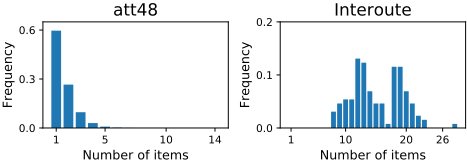
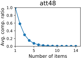
att48 and eil51 are exceptional since the input ZDD is smaller, but D3X is slower than DLX. This result is caused by the difference in subproblems appearing in the search procedure. Figure 4 compares the number of remaining items of subproblems appearing in the recursive calls of SearchZDD on att48 and Interoute. More than 90% of subproblems appearing in att48 have no greater than three items. In contrast, subproblems appearing in Interoute do not show such concentration. This difference affects the running time of D3X since it tends to be slower when the problem is small. Figure 5 shows the average compression ratios of subproblems appearing in the SearchZDD procedure, where we define the compression ratio of a problem as |ZDD|/|DLX|, i.e., the ratio between the number of active node cells of DanceDD and dancing links structures. For example, the compression ratio of the initial problem appearing in Example 1 is 8/13 = 0.615. D3X can be slower than DLX if the compression ratio is high since D3X needs constant time overhead per node cell to update as compared with the number of operations performed in a node cell in the dancing links structure. If an exact cover problem is easy and has many solutions, then the search procedure tends to spend more time solving relatively small subproblems, meaning that DLX will be faster than D3X at solving such problems.
6 RelatedWork
Since the DLX is simple but efficient, it has some extensions. Knuth [Knuth, 2019] shows a few crucial extensions of exact cover problems, including exact cover with colors (XCC) problems and XCC with multiplicity problems. Another extension is made in [Chabert and Solnon, 2020] to cope with different types of constraints. [Nishino et al., 2017] also combines the ZDD with DLX. The algorithm extends DLX to output ZDDs representing the set of solutions of an exact cover problem. Our proposal differs from the previous work in that we try to compress the input of the problem by using a ZDD. Important future work would be to extend the proposed method to combine with these extensions.
How small a ZDD can be depends on the target. Past studies have revealed conditions where the decision diagrams become succinct [Knuth, 2011]. An important target is graph substructures [Kawahara et al., 2017]. Thus, ZDDs and binary decision diagrams [Bryant, 1986] have been used in graph-related problems like network analyses [Hardy et al., 2007], probabilistic inference in a structured space[Choi et al., 2016], and combinatorial optimization [Inoue et al., 2014]. The problems we addressed in the experiments are typical exact cover problems related to graphs.
7 Conclusion
We proposed a problem compression approach for solving an exact cover problem with a huge number of options. Many practical problems can be formulated as an exact cover problem. However, such a reduction might result in an explosion in the problem size. Our DanceDD structure can deal with such size explosion by exploiting ZDDs to represent the problem. The structure inherits the succinctness of the ZDDs while providing low-cost delete and revert operations of the dancing links structure. Using a more compressed representation is another prominent research direction. Zero-suppressed sentential decision diagrams (ZSDDs) [Nishino et al., 2016] are a recently proposed extension of ZDDs. Since ZSDDs can be exponentially smaller than ZDDs, using them instead of ZDDs might incur further acceleration.
Acknowledgements
This work was supported by JSPS KAKENHI Grant Number JP20H05963.
A Details of D3X
We show four subroutines used in CoverZDD(i) and UncoverZDD(i). Algorithm 4 shows the details of CoverLower and UncoverLower, and Alg. 5 shows the details of CoverUpper and UncoverUpper.
CoverLower(C) is used in CoverZDD(i). It updates the node cells that are the descendants of those in C. Since we can make a ZDD that does not contain options having i by removing all high edges of C, we thus update node cells assuming that the high edges of all the node cells in C are removed from the structure. We first create a list of all descendant node cells V , where all cells follow a topological order (line 2). Then, we update plen(p) for all p ∈ V . Since node cells in V are not ancestors of C, we do not need to update the hlen and llen values. Updating all the nodes in V can be done in linear time with |V | via dynamic programming on a directed acyclic graph. We also update len(i) fields as updating plen(p) (line 7). If plen(p) becomes zero, then the node cell should not be accessed from other cells. Therefore, we delete the cell by updating its up, down fields and the parents of child node cells.
UncoverLower(C) in Alg. 4 reverts the modification made by corresponding CoverLower(C). In such a procedure, we have to recover cells in reverse order. Hence, we assume that V is identical to the one appearing in the corresponding CoverLower(C). We store node cells to be restored into a list H (line 21) and restore in the reverse order of H.
Algorithm 4 details the subroutines CoverUpper(C) and UncoverUpper(C). CoverUpper(C) updates the ancestor node cells of C. We first created list V , which stores all the ancestors of C in a reverse topological order (line 2). We then updated llen(p) and hlen(p) for all p ∈ V by assuming that all high edges of node cells in C were removed. We also updated len(i) for i = item(p) so as to reflect the new hlen(p) value (line 8). List H stores all the node cells p whose hlen(p) becomes zero after the update. We finally remove node cell p ∈ H by modifying links (lines 10-18).
UncoverUpper(C) first recovers node cells in list H, which stores the deleted node cells in the corresponding UncoverUpper(C) (lines 21-29). Then, it updates the hlen llen fields of the ancestor node cells of C in a reverse topological order.
Algorithm 4: CoverLower and UncoverLower
1 function CoverLower(C): 2 V ←descendants of C excluding ⊤ in a topological order 3 for p ∈ V do 4 l ← plen(p) 5 Update plen(p) assuming all high edges of q ∈ R were deleted. 6 i ← item(p) 7 len(i) ← len(i) - (l - plen(p)) · hlen(p) 8 if plen(p) = 0 then 9 down(up(p)) ← down(p) 10 up(down(p)) ← up(p) 11 Remove (p, HI) from Parents(hi(p)) 12 Remove (p, LO) from Parents(lo(p)) 13 function UncoverLower(C): 14 V ←descendants of C excluding ⊤ in a topological order 15 H ←empty list 16 for p ∈ V do 17 l ← plen(p) 18 Update plen(p) assuming all high edges of q ∈ C were recovered. 19 i ← item(p) 20 len(i) ← len(i) + (plen(p) - l) · hlen(p) 21 if l = 0 and plen(p) > 0 then Add p to H 22 for p ∈ H (access in a reverse order) do 23 down(up(p)) ← p 24 up(down(p)) ← p 25 Add (p, HI) to Parents(hi(p)) 26 Add (p, LO) to Parents(lo(p))All these subfunctions run in linear time with the number of updated node cells. Thus, the time and space complexity of these procedures are linear with the number of active cells.
@inproceedings{ijcai2021p275,
  title     = {Compressing Exact Cover Problems with Zero-suppressed Binary Decision Diagrams},
  author    = {Nishino, Masaaki and Yasuda, Norihito and Nakamura, Kengo},
  booktitle = {Proceedings of the Thirtieth International Joint Conference on
               Artificial Intelligence, {IJCAI-21}},
  publisher = {International Joint Conferences on Artificial Intelligence Organization},
  editor    = {Zhi-Hua Zhou},
  pages     = {1996--2004},
  year      = {2021},
  month     = {8},
  note      = {Main Track},
  doi       = {10.24963/ijcai.2021/275},
  url       = {https://doi.org/10.24963/ijcai.2021/275},
}
TY - CPAPER TI - Compressing Exact Cover Problems with Zero-suppressed Binary Decision Diagrams AU - Nishino, Masaaki AU - Yasuda, Norihito AU - Nakamura, Kengo T2 - Proceedings of the Thirtieth International Joint Conference on Artificial Intelligence, IJCAI-21 PB - International Joint Conferences on Artificial Intelligence Organization PY - 2021 SP - 1996 EP - 2004 DO - 10.24963/ijcai.2021/275 UR - https://doi.org/10.24963/ijcai.2021/275 ER -Copied
Machine-readable versions of this paper, for tools and AI agents:





