
Physics-informed Spline Learning for Nonlinear Dynamics Discovery
Proceedings of the Thirtieth International Joint Conference on Artificial Intelligence. Main Track. Pages 2054-2061.
https://doi.org/10.24963/ijcai.2021/283
Keywords
- Machine Learning: Learning Sparse Models
- Machine Learning: Explainable/Interpretable Machine Learning
- Knowledge Representation and Reasoning: Leveraging Knowledge and Learning
Abstract
Dynamical systems are typically governed by a set of linear/nonlinear differential equations. Distilling the analytical form of these equations from very limited data remains intractable in many disciplines such as physics, biology, climate science, engineering and social science. To address this fundamental challenge, we propose a novel Physics-informed Spline Learning (PiSL) framework to discover parsimonious governing equations for nonlinear dynamics, based on sparsely sampled noisy data. The key concept is to (1) leverage splines to interpolate locally the dynamics, perform analytical differentiation and build the library of candidate terms, (2) employ sparse representation of the governing equations, and (3) use the physics residual in turn to inform the spline learning. The synergy between splines and discovered underlying physics leads to the robust capacity of dealing with high-level data scarcity and noise. A hybrid sparsity-promoting alternating direction optimization strategy is developed for systematically pruning the sparse coefficients that form the structure and explicit expression of the governing equations. The efficacy and superiority of the proposed method have been demonstrated by multiple well-known nonlinear dynamical systems, in comparison with two state-of-the-art methods.
- [Asseman et al., 2018] Alexis Asseman, Tomasz Kornuta, and Ahmet Ozcan. Learning beyond simulated physics. In Modeling and Decision-making in the Spatiotemporal Domain Workshop-NIPS, 2018.
- [Berg and Nyström, 2019] Jens Berg and Kaj Nyström. Data-driven discovery of PDEs in complex datasets. Jour- nal of Computational Physics, 384:239-252, 2019.
- [Billard and Diday, 2003] L Billard and E Diday. From the statistics of data to the statistics of knowledge: symbolic data analysis. Journal of the American Statistical Associ- ation, 98(462):470-487, 2003.
- [Bongard and Lipson, 2007] Josh Bongard and Hod Lipson. Automated reverse engineering of nonlinear dynamical systems. Proceedings of the National Academy of Sci- ences, 104(24):9943-9948, 2007.
- [Both et al., 2020] Gert-Jan Both, Subham Choudhury, Pierre Sens, and Remy Kusters. DeepMoD: Deep learning for model discovery in noisy data. Journal of Computational Physics, page 109985, 2020.
- [Brunton et al., 2016] Steven L Brunton, Joshua L Proctor, and J Nathan Kutz. Discovering governing equations from data by sparse identification of nonlinear dynamical sys- tems. Proceedings of the National Academy of Sciences, 113(15):3932-3937, 2016.
- [Champion et al., 2019] Kathleen Champion, Bethany Lusch, J Nathan Kutz, and Steven L Brunton. Data- driven discovery of coordinates and governing equations. Proceedings of the National Academy of Sciences, 116(45):22445-22451, 2019.
- [Chen et al., 2020] Zhao Chen, Yang Liu, and Hao Sun. Physics-informed learning of governing equations from scarce data. arXiv preprint arXiv:2005.03448, 2020.
- [Džeroski and Todorovski, 1993] Sašo Džeroski and Ljupéo Todorovski. Discovering dynamics. In Proc. tenth inter- national conference on machine learning, pages 97-103, 1993.
- [Dzeroski and Todorovski, 1995] Saso Dzeroski and Ljupco Todorovski. Discovering dynamics: from inductive logic programming to machine discovery. Journal of Intelligent Information Systems, 4(1):89-108, 1995.
- [Janot et al., 2019] Alexandre Janot, Maxime Gautier, and Mathieu Brunot. Data set and reference models of emps. In Nonlinear System Identification Benchmarks, 2019.
- [Kaheman et al., 2020] Kadierdan Kaheman, J Nathan Kutz, and Steven L Brunton. Sindy-pi: A robust algorithm for parallel implicit sparse identification of nonlinear dynam- ics. arXiv preprint arXiv:2004.02322, 2020.
- [Kaiser et al., 2018] Eurika Kaiser, J Nathan Kutz, and Steven L Brunton. Sparse identification of nonlinear dy- namics for model predictive control in the low-data limit. Proceedings of the Royal Society A, 474(2219):20180335, 2018.
- [Kim et al., 2019] Samuel Kim, Peter Lu, Srijon Mukherjee, Michael Gilbert, Li Jing, Vladimir Ceperic, and Marin Soljacic. Integration of neural network-based symbolic re- gression in deep learning for scientific discovery. arXiv preprint arXiv:1912.04825, 2019.
- [Kingma and Ba, 2014] Diederik P Kingma and Jimmy Ba. Adam: A method for stochastic optimization. arXiv preprint arXiv:1412.6980, 2014.
- [Kubalík et al., 2019] Jiří Kubalík, Jan Žegklitz, Erik Derner, and Robert Babuška. Symbolic regression methods for reinforcement learning. arXiv preprint arXiv:1903.09688, 2019.
- [Long et al., 2019] Zichao Long, Yiping Lu, and Bin Dong. Pde-net 2.0: Learning pdes from data with a numeric- symbolic hybrid deep network. Journal of Computational Physics, 399:108925, 2019.
- [Lorenz, 1963] Edward N Lorenz. Deterministic non- periodic flow. Journal of the Atmospheric Sciences, 20(2):130-141, 1963.
- [Mangan et al., 2016] Niall M Mangan, Steven L Brunton, Joshua L Proctor, and J Nathan Kutz. Inferring biological networks by sparse identification of nonlinear dynamics. IEEE Transactions on Molecular, Biological and Multi- Scale Communications, 2(1):52-63, 2016.
- [Quade et al., 2016] Markus Quade, Markus Abel, Kamran Shafi, Robert K Niven, and Bernd R Noack. Prediction of dynamical systems by symbolic regression. Physical Review E, 94(1):012214, 2016.
- [Rudy et al., 2017] Samuel H Rudy, Steven L Brunton, Joshua L Proctor, and J Nathan Kutz. Data-driven dis- covery of partial differential equations. Science Advances, 3(4):e1602614, 2017.
- [Sahoo et al., 2018] Subham Sahoo, Christoph Lampert, and Georg Martius. Learning equations for extrapolation and control. In International Conference on Machine Learn- ing, pages 4442-4450, 2018.
- [Schaeffer, 2017] Hayden Schaeffer. Learning partial differ- ential equations via data discovery and sparse optimiza- tion. Proceedings of the Royal Society A: Mathematical, Physical and Engineering Sciences, 473(2197):20160446, 2017.
- [Schmidt and Lipson, 2009] Michael Schmidt and Hod Lip- son. Distilling free-form natural laws from experimental data. Science, 324(5923):81-85, 2009.
- [Wang et al., 2016] Wen-Xu Wang, Ying-Cheng Lai, and Celso Grebogi. Data based identification and prediction of nonlinear and complex dynamical systems. Physics Re- ports, 644:1-76, 2016.
- [Zhang and Ma, 2020] Jun Zhang and Wenjun Ma. Data- driven discovery of governing equations for fluid dynam- ics based on molecular simulation. Journal of Fluid Me- chanics, 892:A5, 2020.
References were extracted automatically from the PDF and may contain errors.
Full text extracted automatically from the PDF; figures, tables and equations may differ. The PDF is the version of record.
1 Introduction
Nonlinear dynamics is commonly seen in nature (in many disciplines such as physics, biology, climate science, engineering and and social science), whose behavior can be analytically described by a set of nonlinear governing differential equations, expressed as˙y(t) = F(y(t)) (1)
where y(t) = {y1(t), y2(t), ..., yn(t)} ∈ R1×n denotes the system state at time t, F(·) a nonlinear functional defining the equations of motion and n the system dimension. Note that
∗Corresponding Author
˙y(t) = dy/dt. There remain many underexplored dynamical systems whose governing equations (e.g., the exact or explicit form of F) or physical laws are unknown. For example, the mathematical description of an uncharted biological evolution process might be unclear, which is in critical need for discovery given observational data. Nevertheless, distilling the analytical form of the equations from scarce and noisy data, commonly seen in practice, is an intractable challenge.
Data-driven discovery of dynamical systems dated back decades [Dˇzeroski and Todorovski, 1993; Dzeroski and Todorovski, 1995]. Recent advances in machine learning and data science encourage attempts to develop methods to uncover equations that best describe the underlying governing physical laws. One popular solution relies on symbolic regression with genetic programming [Billard and Diday, 2003], which has been successfully used to distill mathematical formulas (e.g., natural/control laws) that fit data [Bongard and Lipson, 2007; Schmidt and Lipson, 2009; Quade et al., 2016; Kubal´ık et al., 2019]. However, this type of approach does not scale well with the system dimension and generally suffers from extensive computational burden when the dimension is high that results in a large search space. Another progress leverages symbolic neural networks to uncover analytical expressions to interpret data [Sahoo et al., 2018; Kim et al., 2019; Long et al., 2019], where commonly seen mathematical operators are employed as symbolic activation functions to establish intricate formulas through weight pruning. Nevertheless, this existing framework is primarily built on empirical pruning of the weights, thus exhibits sensitivity to user-defined thresholds and may fall short to produce parsimonious equations for complex systems. Moreover, this method requires numerical differentiation of measured system response to feed the network for discovery of dynamics in the form of Eq. (1), leading to substantial inaccuracy especially when the measurement data is sparsely sampled with large noise.
Another alternative approach reconstructs the underlying equations based on a large-space library of candidate terms and eventually turns the discovery problem to sparse regression [Wang et al., 2016; Brunton et al., 2016]. In particular, the breakthrough work [Brunton et al., 2016] introduced a novel paradigm called Sparse Identification of Nonlinear Dynamics (SINDy) for data-driven discovery of governing equations, based on a sequential threshold ridge regression
(STRidge) algorithm which recursively determines the sparse solution subjected to pre-defined or adaptive hard thresholds [Brunton et al., 2016; Rudy et al., 2017; Champion et al., 2019]. This method has drawn tremendous attention in recent years, showing successful applications in biological systems [Mangan et al., 2016], predictive control [Kaiser et al., 2018], continuous systems (described by partial differential equations (PDEs)) [Rudy et al., 2017; Schaeffer, 2017; Zhang and Ma, 2020], etc. Compared with the above symbolic models, SINDy is less computationally demanding thus being more efficient. Nonetheless, since this method relies heavily on the numerical differentiation as target for derivative fitting, it is very sensitive to both data noise and scarcity. Another limitation is that SINDy is unable to handle nonuniformly sampled data while data missing is a common issue in practical applications.
One way to tackle these issues is to build a differentiable surrogate model to approximate the system state which best fits the measurement data meanwhile satisfying the governing equations to be discovered (e.g., by SINDy). Several recent studies [Berg and Nystr¨om, 2019; Chen et al., 2020; Both et al., 2020] have shown that deep neural networks (DNNs) can serve as the approximator where automatic differentiation is used to calculate essential derivatives required for reconstructing the governing PDEs. Nevertheless, since DNNs are rooted in global universal approximation, it is extremely computationally demanding to obtain a fine-tuned model with high accuracy of local approximation (crucial for equation discovery), especially when the nonlinear dynamics is very complex, e.g., chaotic. To overcome this issue, we take advantage of cubic B-splines, a powerful local approximator for time series. Specifically, we develop a Physics Informed Spline Learning (PiSL) approach to discover sparsely represented governing equations for nonlinear dynamics, based on scarce and noisy data. The key concept is to (1) leverage splines to interpolate locally the dynamics, perform analytical differentiation and build the library of candidate terms, (2) reconstruct the governing equations via sparse regression, and (3) use the equation residual as constraint in turn to inform the spline approximation. The synergy between splines and discovered equations leads to the robust capacity of dealing with high-level data scarcity and noise. A hybrid sparsity-promoting alternating direction optimization strategy is developed for systematically training the spline parameters and pruning the sparse coefficients that form the structure and explicit expression of the governing equations. The efficacy of PiSL is finally demonstrated by two chaotic systems under different conditions of data volume and noise.
2 Methodology
In this section, we state and explain the concept and algorithm of PiSL for discovering governing equations for nonlinear dynamics, including introduction to cubic B-Splines, the basic network architecture, and physics-informed network training (in particular, a hybrid sparsity-promoting alternating direction optimization approach).
2.1 Cubic B-Splines
Cubic B-splines, as one type of piece-wise polynomials of degree 3 with continuity at the knots between adjacent segments, have been widely used for curve-fitting and numerical differentiation of experimental data. The basis function N(t) between two knots are defined as:
where τs denotes knot, k denotes degree of polynomial (e.g., k = 3), and t can be any point in the given domain. Cubic Bspline interpolation is calculated by multiplying the values of the nonzero basis functions with a set of equally spaced control points p ∈ R(r+3)×1 , namely, y(t) = ∑r+2 s=0 Ns,3(t)ps, where the number of control points r + 3 is chosen empirically, mainly in accordance with the frequency of system state while accounting for computational efficiency, i.e., small number for smooth response to avoid overfitting and large number for intense oscillation to fully absorb measurement information. The optimal set of control points will produce the splines that best fit the given information (e.g., data). In the case of approximating nonlinear dynamics by cubic Bsplines, we place r+7 knots to cover the calculation of lower degree basis functions, in a non-decreasing order in time domain [0, T ], denoted by τ0, τ1, τ2, ..., τr+6 where τ0 < τ1 < τ2 < τ3 = 0 and τr+3 = T < τr+4 < τr+5 < τr+6. One important feature of cubic B-splines is that the functions are analytically differentiable (e.g., ˙N can be obtained based on Eq. (2)) and and their first and second derivatives are all continuous, which allows us to fit not only data but also the differential equations shown in Eq. (1).
2.2 Network Architecture
We start with an overview of the PiSL network architecture, as depicted in Figure 1. We first define n sets of control points for cubic B-splines P = {p1, p2, ..., pn} ∈ R(r+3)×n , which are multiplied with the spline basis N(t) to interpolate the ndimensional system state:
Thus, we can obtain ˙y(P) = ˙NP based on analytical differentiation. We assume that the form of F(·) in Eq. (1) is governed by only a few important terms which can be selected from a library of l candidate functions φ(y) ∈ R1×l [Brunton et al., 2016] which consists of many candidate terms, e.g., constant, polynomial, trigonometric and other functions :
where ⊙ denotes the element-wise Hadamard product. With the interpolated state variables and their analytical derivatives, the governing equations can be written as:
where φ(P) = φ(y(t; P)); Λ = {λ1, λ2, ..., λn} ∈ Rl×n is the coefficient matrix belonging to a constraint subset S
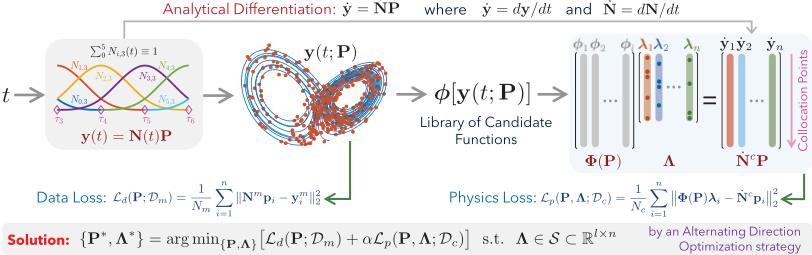
satisfying sparsity (only the active candidate terms in φ have non-zero values), e.g., Λ ∈ S ⊂ Rl×n . Hence, the discovery problem can then be stated as: denoting the measurement domain as m and given the measurement data Dm = {ym i }i=1,...,n ∈ RNm×n , find the best set of P and Λ such that Eq. (5) holds ∀t. Here, ym i is the measured response of the ith state and Nm is the number of data points in the measurement. The loss function for training the PiSL network consists of the data (Ld) and physics (Lp) components, expressed as follows:
where Dc = {t0, t1, ..., tNc-1} denotes the randomly sampled Nc collocation points (Nc ≫ Nm), which are used to enhance the physics satisfaction ∀t (e.g., setting Nc ≥ 10Nm to promote the physics obeyed); Nm ∈ RNm×(r+3) represents the spline basis matrix evaluated at the measured time instances while ˙Nc ∈ RNc×(r+3) is the derivative of the spline basis matrix at the collocation instances; Φ ∈ RNc×l is the collocation library matrix of candidate terms. Mathematically, training the PiSL network is equivalent to solving the following optimization problem:
where α is the relative weighting; S enforces the sparsity of Λ. This constrained optimization problem is solved by the network training strategy discussion in Section 2.3. The synergy between spline interpolation and sparse equation discovery results in the following outcome: the splines provide accurate modeling of the system responses, their derivatives and possible candidate function terms as a basis for constructing the governing equations, while the sparsely represented equations in turn constraints the spline interpolation and project correct candidate functions, eventually turning the measured system into closed-form differential equations.
Remark: Accounting for Multiple Datasets. When multiple independent datasets are available (e.g., due to different initial conditions (ICs)), parallel sets of cubic B-splines are used to approximate the system states corresponding to each dataset. The data loss in Eq. (6) should be defined as the error aggregation over all datasets, while the terms used for assembling the physics loss in Eq. (7) will be stacked since all the system responses satisfy a unified physical law.
2.3 Network Training
The network will be trained through a three-stage strategy discussed herein, including pre-training, sparsity-promoting alternating direction optimization, and post-tuning.
Pre-training
We firstly employ a weakly physics-informed gradient-based optimization to pre-train the network. We call it "weakly physics-informed" because we are not given the governing equations with a concrete (sparse) form. Instead, we define an appropriate library φ that includes all possible terms. This step simultaneously leverages the splines to interpolate the system states and generate a raw solution for nonparsimonious governing equations where the coefficients Λ are not constrained by sparsity. In particular, this is accomplished by a standard gradient descent optimizer like Adam or Adamax [Kingma and Ba, 2014] simultaneously optimizing the trainable variables {P,Λ} in Eq. (8) without imposing the constraint. The outcome of pre-training will lead to a reasonable set of splines, for system state approximation, that not only well fit the data but also satisfy the general form of governing equations shown in Eq. (1).
Sparsity-Promoting Alternating Direction Optimization
Finding the sparsity constraint subset S in Eq. (8) is a notorious challenge. Hence, we turn the constrained optimization to an unconstrained form augmented by an ℓ0 regularizer that enforces the sparsity of Λ. The total loss function reads:
L(P, Λ) = Ld(P; Dm) + αLp(P, Λ; Dc) + β ‖Λ‖0 (9) where β denotes the regularization parameter; ‖·‖0 represents the ℓ0 norm. On one hand, directly solving the optimization problem based on gradient descent is highly intractable since the ℓ0 regularization makes this problem NP-hard. On the other hand, relaxation of ℓ0 to ℓ1 eases the optimization but only loosely promotes the sparsity. To tackle this challenge, we develop a sparsity-promoting alternating direction optimization (ADO) strategy that hybridizes gradient decent optimization and adaptive STRidge [Rudy et al., 2017]. The
Algorithm 1: Hybrid ADO Strategy
1 Input: Library Φ, measurement Dm, collocation points Dc and spline basis N; 2 Parameters: K, δtol,M,R, α, β, η; 3 Output: Best solution ˜Λ⋆ and P⋆ ; 4 Initialize: Λ1, P⋆ = P1 and L⋆ = L(P1, Λ1) from pre-training; 5 for k ← 1 to K do 6 Φ = Φ(P⋆ ); 7 for i ← 0 to n do 8 yi = ˙Ncp⋆i ; 9 λi,k+1 = STRidge(Φ, yi, δtol, M, R, β, η) ; 10 end 11 Eliminate zeros in Λk+1 to form ˜Λ; 12 {Pk+1, ˜Λk+1} = arg min {P, ˜Λ} [Ld(P) +αLp(P, ˜Λ)]; 13 if L(Pk+1, ˜Λk+1) < L⋆ then 14 L⋆ = L(Pk+1, ˜Λk+1); 15 ˜Λ⋆ = ˜Λk+1 and P⋆ = Pk+1; 16 end 17 endconcept is to divide the overall optimization problem into a set of tractable sub-optimization problems, given by:
where k ∈ N is the alternating iteration; ˜Λ consists of only non-zero coefficients in Λk+1 = {λ1,k+1, ..., λn,k+1}; the notations of Dm and Dc are dropped for simplification. The hyper-parameters can be selected following the criteria: β can be estimated by Pareto-front analysis based on pre-trained PiSL; η is a small number (e.g., 10-6 ); and α follows the scale ratio between state and its derivative (e.g., α ∼ [σ(y)/σ( ˙y)]2 ). In each iteration, Λk+1 in Eq. (10) is determined by STRidge with adaptive hard thresholding (e.g., small values are pruned via assigning zero), while Eq. (11) is solved by gradient descent to obtain Pk+1 and ˜Λk+1 with the remaining candidate terms in Φ. Note that each column in Φ is normalized to improve the solution posedness in ridge regression. The process is repeated for multiple (K) iterations until the spline interpolation and pruned equations reach a final balance (e.g., no more pruning is needed). The pseudo codes of this approach are given in Algorithms 1 and 2.
Post-tuning
Once we get the parsimonious form of governing equations from the above ADO process, we post-tune the control points P and non-zero coefficients ˜Λ to make sure the spline interpolation and physical law are consistent. The post-tuning step is similar to pre-training except that the governing equations in post-tuning are comprised of only remaining terms and coefficients. The optimization result out of this post-tuning step is regarded as our final discovery result, where ˜Λ⋆ will be used to reconstruct the explicit form of governing equations.
Algorithm 2: STRidge
1 Input: Library Φ and data y; 2 Parameters: δtol,M,R, β, η; 3 Output: Best solution ˜λ⋆ ; 4 Baseline: ˜λ⋆ = (Φ)-1y, L⋆ = ∥∥Φ˜λ⋆ - y∥∥22 + β∥∥˜λ⋆∥∥0 ; 5 Initialize: tol = δtol,Φ(0) = Φ; 6 for j ← 1 to M do 7 for i ← 1 to R do 8 λ(i) = [ΦT(i-1)Φ(i-1) + ηI ]-1ΦT(i-1)y ; 9 ˜λ(i) = λ(i)[λ(i) ≥ tol]; 10 Φ(i) = Φ(i-1)[λ(i) ≥ tol]; 11 end 12 L = ∥∥Φ(R) ˜λ(R) - y∥∥22 + β∥∥˜λ(R)∥∥0 ; 13 if L < L⋆ then 14 L⋆ = L and ˜λ⋆ = ˜λ(R) ; 15 else 16 δtol = δtol/1.618; 17 end 18 tol = tol + δtol; 19 end3 Numerical Experiments
In this section, we evaluate the efficacy of PiSL in the discovery of governing equations for two nonlinear chaotic dynamical systems based on sparsely sampled synthetic noisy data (e.g., single dataset or multi-source independent datasets, uniformly or non-uniformly sampled) and a system based on experimental data. We also compare the performance of our approach with two open source state-of-art models: GeneticProgramming-based symbolic regression (Eureqa) [Schmidt and Lipson, 2009] and the SINDy method (PySINDy) [Brunton et al., 2016]. The robustness of PiSL against different levels of data noise is analyzed. The discovered equations are further validated on different datasets generated under disparate ICs to show the interpretability and generalizability. The synthetic datasets are generated by solving nonlinear differential equation by the Matlab ode113 function. The proposed computational framework is implemented in PyTorch to leverage the power of graph-based GPU computing. All simulations in this paper are performed on a NVIDIA GeForce RTX 2080Ti GPU in a workstation with 8 Intel Core i9-9900K CPUs 1 .
3.1 Lorenz System
The first example is 3-dimensional Lorenz system [Lorenz, 1963] with its dynamical behavior (x, y, z) governed by
We consider the parameters σ = 10, β = 8/3 and ρ = 28, under which the Lorenz attractor has two lobes and the system, starting from anywhere, makes cycles around one lobe before switching to the other and iterates repeatedly. The resulting system exhibits strong chaos. Gaussian white noise is added to clean signals with the noise level defined as the rootmean-square ratio between the noise and the exact solution. In particular, we consider 5% noise in this example.
1 Source codes/datasets are available on GitHub at https://github. com/isds-neu/PiSL upon final publication.
| Model | Discovered Governing Equations |
|---|---|
| Eureqa | ˙x = -0.56 - 9.02x + 9.01y ˙y = -0.047 + 18.79x + 1.86y - 0.046xy - 0.74xz ˙z = -3.04 - 2.23z + 0.88xy |
| PySINDy | ˙x = -0.46 - 9.18x + 9.17y ˙y = 22.32x + 0.15y - 0.85xz ˙z = 6.04 - 2.83z + 0.15x2 + 0.81xy |
| PiSL | ˙x = -10.06x + 10.03y ˙y = 28.11x - 0.98y - 1.01xz ˙z = -2.66z + 0.99xy |
| True | ˙x = -10x + 10y ˙y = 28x - y - xz ˙z = -2.667z + xy |
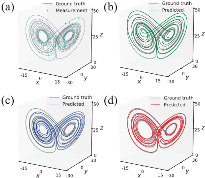
We first generate a single set of data uniformly sampled in [0, 20] sec at 20 Hz. Figure 2a illustrates the ground truth trajectory and the noisy measurement. We discover the equations in Eq. (12) by Eureqa, PySINDy, and PiSL as well as compare their performances. The candidate function library φ ∈ R1×20 used in PySINDy and and PiSL contains all polynomial functions of variables {x, y, z} up to the 3rd degree. The derivatives of system state variables required by Eureqa and PySINDy are numerically approximated and smoothed by Savitzky-Golay filter. The mathematical operators allowed in Eureqa include {+, ×}, where its complexity upper bound is set to be 250. The discovered equations are listed in Table 1 along with their predicted system responses (in a validation setting) shown in Figure 2. It is observed that PiSL uncovers the explicit form of equations accurately in the context of both active terms and coefficients, whereas Eureqa and PySINDy yields several false positives. The trajectory of the attractor is also much better predicted by the PiSL-discovered equations. We conclude that PiSL outperforms PySINDy and Eureqa in this discovery. On the one hand, while both PySINDy and Eureqa rely on numerical differentiation, PiSL is more robust against data scarcity and noise thanks to analytical differentiation. On the other hand, the sparsity-promoting ADO strategy is more reliable for coefficient pruning compared with the sparse identification approach in PySINDy and the insufficiency of adequate sparsity control against data noise in Eureqa, thus producing a more parsimonious solution.
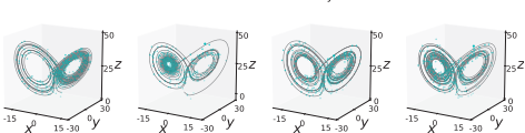
Next, we consider an extended case: we have multi-source measurement datasets for Lorenz attractors that are governed by the same physical law as shown in Eq. (12). Under such a circumstance, these systems, although simulated from different ICs, are in fact homogeneous. We describe their responses with a unified set of governing equations to be uncovered, which are supported by different sets of control points in splines but satisfying same physics. This ought to generate more accurate discovery since the model gathers more information on the underlying physics, despite in the presence of severe scarcity and noise of each dataset. In the following experiment, we challenge PiSL in terms of data quality by nonuniformly sub-sampling (50% of the single dataset), which simulates the scenario of data missing or compressive sensing. We generate the noisy sub-sampled datasets under four different ICs as measurements (see Figure 3) for discovery.
The discovered governing equations by PiSL based on multiple datasets are given by
which are almost identical to the ground truth (see Table 1). Compared with the PiSL-discovered equations in Table 1, we can see that multi-set measurements help improve the discovery accuracy, despite the fact that the data quality and quantity of each measured attractor is worse than that in the single-set case. We conclude that, even though measurements are randomly sampled, causing the missing data issue, PiSL is still able to recapitulate the state variables through spline learning, meanwhile taking advantage of richer information from multi-set measurements to generate more accurate and less biased discovery of the governing equation for the chaotic dynamical system.
3.2 Double Pendulum System
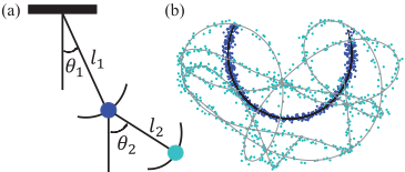
Our second numerical experiment is another chaotic system, double pendulum, as shown in Figure 4, which exhibits rich dynamic behavior with a strong sensitivity to ICs. In this system, one pendulum (m1) is attached to an fixed end by a rod with length l1, while another pendulum (m2) is attached to the first one by a rod with length l2. This is a classic yet challenging problem for equation discovery [Schmidt and Lipson, 2009; Kaheman et al., 2020]. The system behavior is governed by two second-order differential equations with angles θ1 and θ2 as the state variables (see Figure 4). These equations can be derived by the Lagrangian method:
where ω1 = ˙ θ1 and ω2 = ˙ θ2; g denotes the gravity constant. We can see the nonlinearity from the above equations, which yield complicated behavior of the two pendulums. In fact, the behavior of this system is extremely chaotic and sensitive to the coefficients in the equations, which can be recapitulated only by the precise form of equations. We herein apply PiSL to discover the equations of motion shown in Eq. (14) based on measured noisy trajectories.
In order to simulate a real-world situation, we consider the following parameters for a double pendulum system which match an experimental setting [Asseman et al., 2018]: m1 = 35 g, m2 = 10 g, l1 = 9.1 cm, l2 = 7 cm, with the IC of θ1 = 1.951 rad, θ2 = -0.0824 rad, ω1 = -5 rad/s and ω2 = -1 rad/s. Since the angles are not directly measurable, we generate the synthetic time histories of {θ1, θ2} and convert them to trajectories of the two pendulums, e.g., {x1, y1} and {x2, y2}. We measure these trajectories (e.g., by video camera in practice) for 2 seconds with a sampling rate of 800 Hz and then transform back to angular time histories as measurement data for discovery. Three different noise conditions (e.g., 0% or noise-free, 2% and 5%) and two subsampling frequencies (400 Hz and 200 Hz) are considered to test the robustness of PiSL and PySINDy against measurement noise and sparsity, which imitate the errors due to various precision of camera experiment setup. For this double pendulum system, we define a candidate library φ with 20 candidate terms for both models:
| Data | Discovered Governing Equations |
|---|---|
| 0% 400Hz | ˙ω1 = -0.170 ˙ω2 cos(Δθ) - 0.171ω2 2 sin(Δθ) - 107.80 sin(θ1) ˙ω2 = -1.294 ˙ω1 cos(Δθ) + 1.302ω2 1 sin(Δθ) - 139.80 sin(θ2) |
| 2% 400Hz | ˙ω1 = -0.170 ˙ω2 cos(Δθ) - 0.171ω2 2 sin(Δθ) - 107.80 sin(θ1) ˙ω2 = -1.280 ˙ω1 cos(Δθ) + 1.310ω2 1 sin(Δθ) - 138.04 sin(θ2) |
| 5% 400Hz | ˙ω1 = -0.170 ˙ω2 cos(Δθ) - 0.169ω2 2 sin(Δθ) - 107.80 sin(θ1) ˙ω2 = -1.310 ˙ω1 cos(Δθ) + 1.300ω2 1 sin(Δθ) - 140.59 sin(θ2) |
| 0% 200Hz | ˙ω1 = -0.170 ˙ω2 cos(Δθ) - 0.171ω2 2 sin(Δθ) - 107.81 sin(θ1) ˙ω2 = -1.263 ˙ω1 cos(Δθ) + 1.314ω2 1 sin(Δθ) - 136.65 sin(θ2) |
| True | ˙ω1 = -0.171 ˙ω2 cos(Δθ) - 0.171ω2 2 sin(Δθ) - 107.80 sin(θ1) ˙ω2 = -1.300 ˙ω1 cos(Δθ) + 1.300ω2 1 sin(Δθ) - 140.14 sin(θ2) |
| Data | Model | Target Terms Found? | False Positives |
|---|---|---|---|
| 0% | PiSL | Yes | 0 |
| 400Hz | PySINDy | Yes | 3 |
| 2% | PiSL | Yes | 0 |
| 400Hz | PySINDy | No | NA |
| 5% | PiSL | Yes | 0 |
| 400Hz | PySINDy | No | NA |
| 0% | PiSL | Yes | 0 |
| 200Hz | PySINDy | Yes | 3 |
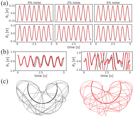
where Δθ = θ1 - θ2, φθ = {sin(θ1), sin(θ2), sin(Δθ)} and φω = {1, ω1, ω2, ω2 1 , ω2 2 , ω1ω2}. The PiSL-discovered equations, in comparison with the ground truth for this double pendulum system, are shown in Table 2. The effects of data noise and sampling frequency on discovery the accuracy of PiSL and PySINDy are shown in Table 3. The closed-form expressions are successfully uncovered by PiSL with accurately identified coefficients in all data conditions considered herein, while PySINDy exhibits weaker sparsity control (e.g., yielding false positives) in the cases of noiseless datasets and evidently suffers from data noise. For validation of the PiSLdiscovered equations, we consider two cases: (1) a small IC leading to periodic oscillation for both pendulums, where θ1 and θ2 never exceed the base range [-π, π]; (2) a large IC causing chaotic behavior of the second pendulum, where θ2 exceeds [-π, π]. The validation result is depicted in Figure 5a for small IC and in Figure 5b-c for large IC. It is seen that, although the small oscillations can be well predicted, the chaotic behavior is intractable to recapitulate (only the dynamics within the first second is accurately captured). This is due to the fact that, for ICs which are large enough to cause chaos, the response is extremely sensitive to the equation coefficients, even in the presence of a tiny difference.
3.3 Electro-Mechanical Positioning System
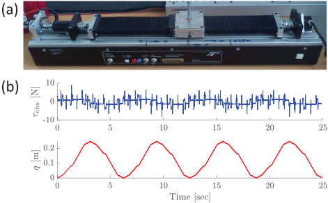
An experimental example is finally considered in this case, aka., an Electro-Mechanical Positioning System (EMPS) [Janot et al., 2019], shown in Fig. 6a, which is a standard configuration of a drive system for prismatic joint of robots or machine tools. The main source of nonlinearity is caused by the friction-dominated energy dissipation mechanism. A possible continuous-time model suitable to describe the forced vibration of this nonlinear dynamical system is given by:
where q (the output), ˙ q and ¨ q are the joint position, velocity and acceleration, respectively; τidm is the joint torque/force (the input); c is a constant offset; M, Fv and Fc are referred to as constant parameters. We introduce a variable p = ˙ q denoting velocity to convert Eq. (16) to the target form of first-order differential equation in a state-space formulation. Fig. 6b shows the measurement data.
We define the candidate library as {q, q2 , p, p2 , sign(p), τ, 1} for PiSL and PySINDy, while allowing {+, ×, sign} and constant as the candidate operations in genetic expansion and set upper bound of complexity to be 50 in the Eureqa approach. The discovery results are reported in Table 4, in comparison with a reference target equation where the values of coefficients are found in [Janot et al., 2019]. We observe that PiSL and Eureqa produce the same equation form with close parameter estimation while PySINDy fails to enforce sparsity in the distilled equation. Given the sparse data, the p2 term in the discovered equations by PiSL and Eureqa supersedes the small offset constant that has a minor effect.
| Model | Discovered Governing Equations |
|---|---|
| Eureqa | ˙p = 0.368τ - 2.248p - 0.202sign(p) + 0.0141 + 2.453p2 |
| PySINDy | ˙p = 0.368τ - 0.112p - 0.212sign(p) + 0.0195 - 2.144q + 0.294p2 + 2.547q2 |
| PiSL | ˙p = 0.369τ - 2.276p - 0.20sign(p) + 0.0121 + 2.547p2 |
| Reference | ˙p = 0.370τ + 2.140p + 0.214sign(p) + 0.0333 |
4 Conclusion
In this paper, we propose a physics-informed spline learning method to tackle the challenge of distilling analytical form of governing equations for nonlinear dynamics from very limited and noisy measurement data. This method takes advantage of spline interpolation to locally sketch the system responses and performs analytical differentiation to feed the physical law discovery in a synergistic manner. Beyond this point, we define the library of candidate terms for sparse representation of the governing equations and use the physics residual in turn to inform the spline learning. We must acknowledge that our approach also has some limitations, e.g, (1) limited capacity of linear combination of candidate functions to represent very complex equations, (2) incorrect discovery given improperly designed library, and (3) inapplicable to problems where system states are incompletely measured or unmeasured. Despite these limitations, the synergy between splines and sparsity-promoting physics discovery leads to a robust capacity for handling scarce and noisy data. Numerical experiments have been conducted to evaluate our method on two classic chaotic systems with synthetic datasets and one system with experimental dataset. Our proposed model outperforms the state-of-the-art methods by a noticeable margin and conveys great efficacy under various high-level data scarcity and noise situations.
@inproceedings{ijcai2021p283,
  title     = {Physics-informed Spline Learning for Nonlinear Dynamics Discovery},
  author    = {Sun, Fangzheng and Liu, Yang and Sun, Hao},
  booktitle = {Proceedings of the Thirtieth International Joint Conference on
               Artificial Intelligence, {IJCAI-21}},
  publisher = {International Joint Conferences on Artificial Intelligence Organization},
  editor    = {Zhi-Hua Zhou},
  pages     = {2054--2061},
  year      = {2021},
  month     = {8},
  note      = {Main Track},
  doi       = {10.24963/ijcai.2021/283},
  url       = {https://doi.org/10.24963/ijcai.2021/283},
}
TY - CPAPER TI - Physics-informed Spline Learning for Nonlinear Dynamics Discovery AU - Sun, Fangzheng AU - Liu, Yang AU - Sun, Hao T2 - Proceedings of the Thirtieth International Joint Conference on Artificial Intelligence, IJCAI-21 PB - International Joint Conferences on Artificial Intelligence Organization PY - 2021 SP - 2054 EP - 2061 DO - 10.24963/ijcai.2021/283 UR - https://doi.org/10.24963/ijcai.2021/283 ER -Copied
Machine-readable versions of this paper, for tools and AI agents:





