
Time-Aware Multi-Scale RNNs for Time Series Modeling
Proceedings of the Thirtieth International Joint Conference on Artificial Intelligence. Main Track. Pages 2285-2291.
https://doi.org/10.24963/ijcai.2021/315
Keywords
- Machine Learning: Deep Learning
- Machine Learning: Time-series; Data Streams
Abstract
Multi-scale information is crucial for modeling time series. Although most existing methods consider multiple scales in the time-series data, they assume all kinds of scales are equally important for each sample, making them unable to capture the dynamic temporal patterns of time series. To this end, we propose Time-Aware Multi-Scale Recurrent Neural Networks (TAMS-RNNs), which disentangle representations of different scales and adaptively select the most important scale for each sample at each time step. First, the hidden state of the RNN is disentangled into multiple independently updated small hidden states, which use different update frequencies to model time-series multi-scale information. Then, at each time step, the temporal context information is used to modulate the features of different scales, selecting the most important time-series scale. Therefore, the proposed model can capture the multi-scale information for each time series at each time step adaptively. Extensive experiments demonstrate that the model outperforms state-of-the-art methods on multivariate time series classification and human motion prediction tasks. Furthermore, visualized analysis on music genre recognition verifies the effectiveness of the model.
- [Bagnall et al., 2018] Anthony Bagnall, Hoang Anh Dau, Ja- son Lines, Michael Flynn, James Large, Aaron Bostrom, Paul Southam, and Eamonn Keogh. The uea multivari- ate time series classification archive, 2018. arXiv preprint arXiv:1811.00075, 2018.
- [Campos et al., 2018] Víctor Campos, Brendan Jou, Xavier Giró-i Nieto, Jordi Torres, and Shih-Fu Chang. Skip rnn: Learning to skip state updates in recurrent neural net- works. In International Conference on Learning Repre- sentations, 2018.
- [Carta et al., 2020] Antonio Carta, Alessandro Sperduti, and Davide Bacciu. Incremental training of a recurrent neural network exploiting a multi-scale dynamic memory. arXiv preprint arXiv:2006.16800, 2020.
- [Chang et al., 2017] Shiyu Chang, Yang Zhang, Wei Han, Mo Yu, Xiaoxiao Guo, Wei Tan, Xiaodong Cui, Michael Witbrock, Mark A Hasegawa-Johnson, and Thomas S Huang. Dilated recurrent neural networks. In Advances in neural information processing systems, pages 77-87, 2017.
- [Chiu et al., 2019] Hsu-kuang Chiu, Ehsan Adeli, Borui Wang, De-An Huang, and Juan Carlos Niebles. Action- agnostic human pose forecasting. In 2019 IEEE Winter Conference on Applications of Computer Vision (WACV), pages 1423-1432. IEEE, 2019.
- [Cui et al., 2016] Zhicheng Cui, Wenlin Chen, and Yixin Chen. Multi-scale convolutional neural networks for time series classification. arXiv preprint arXiv:1603.06995, 2016.
- [Defferrard et al., 2016] Michaël Defferrard, Kirell Benzi, Pierre Vandergheynst, and Xavier Bresson. Fma: A dataset for music analysis. arXiv preprint arXiv:1612.01840, 2016.
- [Fragkiadaki et al., 2015] Katerina Fragkiadaki, Sergey Levine, Panna Felsen, and Jitendra Malik. Recurrent network models for human dynamics. In Proceedings of the IEEE International Conference on Computer Vision, pages 4346-4354, 2015.
- [Hu et al., 2019] Hao Hu, Liqiang Wang, and Guo-Jun Qi. Learning to adaptively scale recurrent neural networks. In Proceedings of the AAAI Conference on Artificial Intelli- gence, volume 33, pages 3822-3829, 2019.
- [Ionescu et al., 2013] Catalin Ionescu, Dragos Papava, Vlad Olaru, and Cristian Sminchisescu. Human3. 6m: Large scale datasets and predictive methods for 3d human sens- ing in natural environments. IEEE transactions on pat- tern analysis and machine intelligence, 36(7):1325-1339, 2013.
- [Jain et al., 2016] Ashesh Jain, Amir R Zamir, Silvio Savarese, and Ashutosh Saxena. Structural-rnn: Deep learning on spatio-temporal graphs. In Proceedings of the ieee conference on computer vision and pattern recogni- tion, pages 5308-5317, 2016.
- [Jernite et al., 2016] Yacine Jernite, Edouard Grave, Ar- mand Joulin, and Tomas Mikolov. Variable compu- tation in recurrent neural networks. arXiv preprint arXiv:1611.06188, 2016.
- [Karim et al., 2019] Fazle Karim, Somshubra Majumdar, Houshang Darabi, and Samuel Harford. Multivariate lstm-fcns for time series classification. Neural Networks, 116:237-245, 2019.
- [Kingma and Ba, 2014] Diederik P Kingma and Jimmy Ba. Adam: A method for stochastic optimization. arXiv preprint arXiv:1412.6980, 2014.
- [Koutnik et al., 2014] Jan Koutnik, Klaus Greff, Faustino Gomez, and Juergen Schmidhuber. A clockwork rnn. In International Conference on Machine Learning, pages 1863-1871, 2014.
- [Martinez et al., 2017] Julieta Martinez, Michael J Black, and Javier Romero. On human motion prediction using recurrent neural networks. In Proceedings of the IEEE Conference on Computer Vision and Pattern Recognition, pages 2891-2900, 2017.
- [Mozer, 1992] Michael C Mozer. Induction of multiscale temporal structure. In Advances in neural information pro- cessing systems, pages 275-282, 1992.
- [Neil et al., 2016] Daniel Neil, Michael Pfeiffer, and Shih- Chii Liu. Phased lstm: Accelerating recurrent network training for long or event-based sequences. Advances in neural information processing systems, 29:3882-3890, 2016.
- [Schäfer and Leser, 2017] Patrick Schäfer and Ulf Leser. Multivariate time series classification with weasel+ muse. arXiv preprint arXiv:1711.11343, 2017.
- [Shokoohi-Yekta et al., 2015] Mohammad Shokoohi-Yekta, Jun Wang, and Eamonn Keogh. On the non-trivial general- ization of dynamic time warping to the multi-dimensional case. In Proceedings of the 2015 SIAM international con- ference on data mining, pages 289-297. SIAM, 2015.
- [Srivastava et al., 2014] Nitish Srivastava, Geoffrey Hinton, Alex Krizhevsky, Ilya Sutskever, and Ruslan Salakhutdi- nov. Dropout: a simple way to prevent neural networks from overfitting. The journal of machine learning re- search, 15(1):1929-1958, 2014.
- [Tamkin et al., 2020] Alex Tamkin, Dan Jurafsky, and Noah Goodman. Language through a prism: A spectral approach for multiscale language representations. Advances in Neu- ral Information Processing Systems, 33, 2020.
- [Wolter and Yao, 2018] Moritz Wolter and Angela Yao. Complex gated recurrent neural networks. Advances in Neural Information Processing Systems, 31:10536-10546, 2018.
- [Zhang et al., 2020] Xuchao Zhang, Yifeng Gao, Jessica Lin, and Chang-Tien Lu. Tapnet: Multivariate time se- ries classification with attentional prototypical network. In AAAI, pages 6845-6852, 2020.
References were extracted automatically from the PDF and may contain errors.
Full text extracted automatically from the PDF; figures, tables and equations may differ. The PDF is the version of record.
1 Introduction
Time series is a set of values sequentially recorded over time. Modeling of time series can provide meaningful knowledge, which is beneficial for decision-making in a variety of fields, such as human motion prediction [Martinez et al., 2017] and EEG/ECG data analysis [Bagnall et al., 2018].
Multi-scale information is crucial to the modeling of time series [Mozer, 1992; Koutnik et al., 2014]. Currently, most methods use multi-scale convolution [Cui et al., 2016] or skip connections to model multiple scales of time series [Koutnik et al., 2014; Chang et al., 2017; Chiu et al., 2019; Carta et al., 2020]. Multi-scale convolution uses different downsampling frequencies or convolution kernels of different sizes, while models with skip connections capture multiple scales through direct connections spanning different lengths. These methods use pre-fixed multiple scales, assuming that all the scales are equally important for each sample.
∗Qianli Ma is the corresponding author.
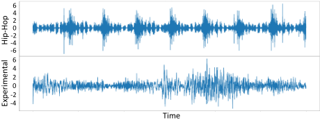
However, it is difficult for these fixed-scale methods to capture the dynamic temporal patterns of time series. For example, Fig. 1 shows two music clips of different genres. "Hip-Hop" is a style of music with a strong beat, while "Experimental" is relatively chaotic. Intuitively, "Hip-Hop" requires a larger scale to capture long-term dependencies due to its regularity, while "Experimental" needs a smaller scale to capture short-term dependencies due to its sharp fluctuations. Hence, we need to adaptively select a suitable scale for each sample rather than a fixed one. Meanwhile, the recognition of genres requires modeling the emotional changes in music, which are controlled by note duration. Therefore, different scales are also needed at different time steps as the notes have different durations at different times [Hu et al., 2019].
Recently, some methods have been proposed to select appropriate scales corresponding to each sample dynamically [Neil et al., 2016; Jernite et al., 2016; Campos et al., 2018; Hu et al., 2019]. These methods select a specific scale adaptively or decide whether to update the hidden state at each time step of the Recurrent Neural Network (RNN). However, these methods attempt to use uniform feature representations to model multiple scales, entangling representations of different scales. It is hard to explore the impact of different scales using the entangled representation, which is harmful to the interpretability of the model [Tamkin et al., 2020]. Hence, disentangling the scales helps learning the representations of different scales better and is conducive to interpretability.
To address the above issues, we propose Time-Aware Multi-Scale RNNs (TAMS-RNNs) that can adaptively model the multi-scale information for each time series at each time step. First, we design a mechanism called Multi-Scale Feature Disentanglement (MSFD) to obtain decoupled feature representations of different scales. Concretely, the hidden state of the RNN is disentangled into multiple independently updated small hidden states, which use different update frequencies to model the multi-scale information. Furthermore, a mechanism called Time-Aware Feature Modulation (TAFM) is designed to modulate the features of different scales, adaptively selecting the most important scale at each time step. We conduct comparative experiments on Multivariate Time Series (MTS) classification, human motion prediction, and music genre recognition to verify the superiority of TAMS-RNNs. The contributions of our work are:
- We propose Time-Aware Multi-Scale RNNs (TAMSRNNs) to adaptively model the multi-scale information for time series modeling. It uses a Multi-Scale Feature Disentanglement (MSFD) mechanism to disentangle feature representations of different scales.
- We design a simple but effective mechanism we call Time-Aware Feature Modulation (TAFM) that uses temporal context information to modulate the features of different scales, adaptively selecting the most important scale for each sample at each time step.
- We conduct extensive experiments showing that our model outperforms state-of-the-art methods on MTS classification and human motion prediction tasks. Furthermore, we visualize the network's behavior on music genre recognition, verifying the model's effectiveness.
2 RelatedWork
Many methods have been proposed that use RNNs to model multi-scale time series dynamics. They can be roughly divided into two categories:
Pre-fixedmulti-scale. ClockworkRNN (CW-RNN) [Koutnik et al., 2014] divides one layer of the RNN into separate modules, each processing inputs at its own temporal granularity. Dilated RNN [Chang et al., 2017] extracts the representations of multiple scales by stacking multiple layers of RNNs and using skip connections of different lengths. MS-LMN [Carta et al., 2020] separates the RNN into different modules with different sampling rates, using an incremental training algorithm to learn long-term dependencies. However, these methods use fixed, predefined scales, making it difficult to adapt to different time series dynamics.
Learnable multi-scale. There are also methods that select suitable scales dynamically. Phased LSTM [Neil et al., 2016] and Skip RNN [Campos et al., 2018] decide whether to update the hidden state at each time step of the RNN to learn representations at multiple scales. VCRNN [Jernite et al., 2016] adaptively determines the number of neurons to be updated at each time step. ASRNN [Hu et al., 2019] presets multiple scales and selects a specific scale at each time step. However, these methods attempt to use uniform feature representations to model multiple scales, and the information of various scales are entangled together. Hence, it is difficult to explore the impact of different scales on the model.
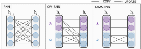
The most relevant model to ours is CW-RNN [Koutnik et al., 2014]. However, in CW-RNN, representations of different scales are entangled together, and it is difficult for the model to capture the dynamic temporal patterns of time series. We update the small hidden states independently to learn the representations of different scales better. Meanwhile, the temporal context information is used to select the most important scale at each time step adaptively, capturing more complicated temporal patterns. A detailed comparison of their update process to ours is shown in Fig. 3.
3 Time-Aware Multi-Scale RNNs
We propose Time-Aware Multi-Scale RNNs (TAMS-RNNs) and design two mechanisms (named Multi-Scale Feature Disentanglement and Time-Aware Feature Modulation, respectively) for TAMS-RNNs to adaptively model the multi-scale information for time series modeling. The whole architecture of TAMS-RNNs is shown in Fig. 2.
3.1 Multi-Scale Feature Disentanglement
Given time series X = {x1, x2, · · · , xT } where xt ∈ Rd0 , d0 is the dimension of input data and T denotes the length of time series, the hidden state ht ∈ Rd of RNN cell can be expressed as follows:
where xt and ht are the input and hidden state at time step t, respectively. W ∈ Rd×d0 , U ∈ Rd×d , and b ∈ Rd are the learnable parameters. f denotes the hyperbolic tangent activation function tanh.
To capture the feature representations of different scales, the mechanism of MSFD is designed. First, the hidden state of RNN is disentangled into multiple small hidden states that are updated independently. Specifically, the hidden state at time step t is disentangled into K small hidden states as ht = [h1t , · · · , hKt ], where hkt ∈ Rp , p = d/K and [·] is the concatenation operation. The corresponding recurrent matrix is defined as ˜U = [ ˜U1 , · · · , ˜UK ], where ˜Uk ∈ Rp×p . Each small hidden state hkt is independently updated by an individual recurrent matrix ˜Uk and then merged via concatenation to constitute the hidden state ht. Meanwhile, The learnable parameter W is defined as W = [W1 , · · · ,WK ], where Wk ∈ Rp×d0 . The update equation of ht is defined as:
where f denotes the hyperbolic tangent activation function tanh and ˜b ∈ Rp is the learnable parameter. Specifically, the model is equivalent to RNNwhen K = 1.
After the disentangling process, each small hidden state would use a specific update frequency to capture information of a particular scale. Suppose the scale set S is {s1, · · · , sK}, for simplicity, sk is usually set to a power of 2 in our experimentation. For scale sk, the small hidden state hkt will be updated every sk time steps. As shown in Fig. 2, the entire hidden state of RNN is disentangled into 3 small hidden states, and the corresponding scale set is {1, 2, 4}. Scale s1
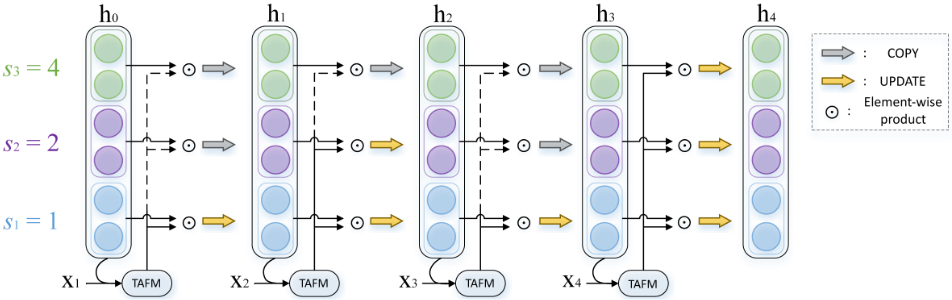
means the small hidden state is updated every time step, while the hidden state of scale s3 is updated every four time steps. Specifically, the update equation of hkt is defined as follow:
When t MOD sk ̸= 0, the "COPY" operation is used, directly copying the hidden state at the last time step. Otherwise, the "UPDATE" operation is employed, using the equation (2) to update the hidden state. After disentangling the hidden state with different update frequencies, each small hidden state is able to capture information of a certain scale. The hidden state with a small scale captures the short-term dependencies, which is crucial for the time series where the values change frequently. Meanwhile, the hidden state with a large scale captures the long-term dependencies, which provides essential information to time series modeling tasks.
Furthermore, we compare the update process of the proposed TAMS-RNN with RNN and CW-RNN [Koutnik et al., 2014], which is shown in Fig. 3. Firstly, compared to RNN, CW-RNN and TAMS-RNN separate the hidden state of RNN into multiple small hidden states, using different update frequencies to capture the multi-scale information of time series. However, in CW-RNN, representations of different scales are entangled together. For example, the hidden state of scale s2
will affect the update process of the small-scale hidden state. Compared to CW-RNN, TAMS-RNN updates the small hidden states independently to learn the representations of corresponding scales better and is also conducive to the interpretability of the model [Tamkin et al., 2020].
3.2 Time-Aware Feature Modulation
After the proposed MSFD, the model still uses multiple fixed scales, which is difficult to capture the dynamic temporal patterns of time series. For example, as shown in Fig. 1, the temporal patterns of two music clips are quite different, and even the patterns of different time steps within the same music series are also different. Therefore, different temporal scales are needed to model the corresponding patterns. To solve the problem, we design a simple but effective mechanism named TAFM that uses temporal context information to modulate the features of different scales so that the model can focus on different scales at different time steps.
First, the temporal context information ht-1 and xt are utilized to generate the distribution αt for each time step:
where αt ∈ RK indicates the importance degree of K small hidden states, and the value of αk t is in the range of 0 to 1. W′ ∈ RK×d0 , U′ ∈ RK×d and b′ ∈ RK are learnable parameters. A larger αk t means that the small hidden state of scale sk is more important for current time step. Then, αt is utilized to modulate the features of different scales, and the update equation of hkt is changed to:
Specially, when the "COPY" operation is used, hkt-1 is not multiplied by αk t , because continuously multiplying by values less than 1 will make the value of feature close to zero, which will lead to gradient vanishing problem. Thus, αk t is utilized to weight hkt-1 only when the "UPDATE" operation is used. After modulating the features of different scales, the model can adaptively select the most important scale at each time step and capture more complex dynamic temporal patterns.
| Data set | TAMS -LSTM | CW -LSTM | TapNet | MLSTM -FCN | WEASEL +MUSE | ED -1NN | DTW -1NN-I | DTW -1NN-D |
|---|---|---|---|---|---|---|---|---|
| ArticularyWordRecognition | 0.973 | 0.947 | 0.987 | 0.973 | 0.990 | 0.970 | 0.980 | 0.987 |
| AtrialFibrillation | 0.400 | 0.333 | 0.333 | 0.267 | 0.333 | 0.267 | 0.267 | 0.200 |
| BasicMotions | 1.000 | 1.000 | 1.000 | 0.950 | 1.000 | 0.675 | 1.000 | 0.975 |
| CharacterTrajectories | 0.994 | 0.990 | 0.997 | 0.985 | 0.990 | 0.964 | 0.969 | 0.990 |
| FaceDetection | 0.602 | 0.594 | 0.556 | 0.545 | 0.545 | 0.519 | 0.513 | 0.529 |
| HandMovementDirection | 0.473 | 0.473 | 0.378 | 0.365 | 0.365 | 0.279 | 0.306 | 0.231 |
| Heartbeat | 0.756 | 0.722 | 0.751 | 0.663 | 0.727 | 0.620 | 0.659 | 0.717 |
| MotorImagery | 0.590 | 0.520 | 0.590 | 0.510 | 0.500 | 0.510 | 0.390 | 0.500 |
| NATOPS | 0.956 | 0.950 | 0.939 | 0.889 | 0.870 | 0.860 | 0.850 | 0.883 |
| PEMS-SF | 0.890 | 0.890 | 0.751 | 0.699 | N/A | 0.705 | 0.734 | 0.711 |
| Pen Digits | 0.981 | 0.976 | 0.980 | 0.978 | 0.948 | 0.973 | 0.939 | 0.977 |
| Phoneme | 0.203 | 0.178 | 0.175 | 0.110 | 0.190 | 0.104 | 0.151 | 0.151 |
| SelfRegulationSCP2 | 0.561 | 0.544 | 0.550 | 0.472 | 0.460 | 0.483 | 0.533 | 0.539 |
| SpokenArabicDigits | 0.990 | 0.986 | 0.983 | 0.990 | 0.982 | 0.967 | 0.960 | 0.963 |
| StandWalkJump | 0.400 | 0.333 | 0.400 | 0.067 | 0.333 | 0.200 | 0.333 | 0.200 |
| No. best | 13 | 3 | 4 | 1 | 2 | 0 | 1 | 0 |
| Best rate | 0.867 | 0.200 | 0.267 | 0.067 | 0.133 | 0 | 0.067 | 0 |
Since our model is based on vanilla RNN, the recurrent cell of TAMS-RNN can be easily replaced with Long Short-Term Memory (LSTM) and Gated Recurrent Units (GRU), which we refer to as TAMS-LSTM and TAMS-GRU.
4 Experiments
Experiments are conducted on MTS classification, human motion prediction and music genre recognition to verify the superiority of the model.
4.1 Multivariate Time Series Classification
Following TapNet [Zhang et al., 2020], we conduct experiments on 15 data sets from the latest MTS classification archive [Bagnall et al., 2018]. These data sets come from various fields with different numbers of classes and variables. Classification accuracy is computed as the evaluation metric.
For MTS classification, following previous work, we use LSTM as the recurrent cell of our model. The number of layers of TAMS-LSTM is set to 2, the hidden state dimension is set to 256 (d = 256), and the hidden state of the final time step is used for classification. Meanwhile, the number of small hidden states is set to 4(K = 4) with the scale set {1, 2, 4, 8}. We apply the dropout operation [Srivastava et al., 2014] to the input time series X with dropout rate of 0.1. The gradient-based optimizer Adam [Kingma and Ba, 2014] is chosen, and the learning rate is set to be 0.001.
We compare the proposed model with six benchmark methods, including deep learning methods (MLSTM-FCN [Karim et al., 2019] and TapNet [Zhang et al., 2020]), bag-of-patterns method (WEASEL+MUSE [Sch¨afer and Leser, 2017]), and common distance-based methods (ED/DTW-NN [ShokoohiYekta et al., 2015]). To fairly compare TAMS-LSTM with CW-RNN [Koutnik et al., 2014], we design a baseline model called "CW-LSTM", replacing the RNN cell of CW-RNN with LSTM. The experiment result is shown in Table 1. The result "N/A" in the table indicates the corresponding approach is unable to run because of computational issues. Meanwhile, the best rate of each model is computed and shown to better describe the performance of these models. The performance comparison shows that TAMS-LSTM outperforms other methods on 13 out of 15 MTS classification data sets and yields the highest best rate of 0.867, which is significantly better than the existing state-of-the-art approach TapNet with the best rate of 0.267. In addition, TAMS-LSTM is also significantly better than CW-LSTM, which illustrates the effectiveness of MSFD and TAFM.
4.2 HumanMotion Prediction
In addition to these 15 MTS data sets, we also conduct experiments on human motion prediction, using the Human 3.6M (H3.6M) data set [Ionescu et al., 2013]. H3.6M is one of the largest publicly available data sets of human motion capture, including seven actors performing 15 activities. Following previous work [Jain et al., 2016; Martinez et al., 2017], we use six actors for training and the actor five for testing. Meanwhile, we train our model for long-term prediction, forecasting the future 25 frames (1000ms). The error is measured by the euclidean distance between the predicted sequences and ground truth, in terms of the Euler angles.
For human motion prediction, RRNN [Martinez et al., 2017] is first proposed, using a sequence-to-sequence architecture with residual connections, which results in much more accurate prediction results. Therefore, under the architecture of RRNN, we replace the vanilla GRU in RRNN with the proposed TAMS-GRU (refer to as TAMS-RRNN) to model the multi-scale information existing in skeleton-based action sequences, such as movements of different amplitudes. Meanwhile, we also compare the proposed model with LSTM3LR [Fragkiadaki et al., 2015] and cgRNN [Wolter and Yao, 2018]. Finally, since TP-RNN [Chiu et al., 2019] is a recently proposed advanced model based on recurrent architecture, we also replace the vanilla LSTM in TP-RNN with the proposed TAMS-LSTM (refer to as TAMS-TP-RNN) to further verify the effectiveness of the proposed model. Since RRNN [Martinez et al., 2017] and cgRNN [Wolter and Yao, 2018] are only trained for short-term prediction (up to 400ms), we train their models for long-term prediction (up to 1000ms) using the publicly available implementations 1 . In TAMS-RRNN and TAMS-TP-RNN, the number of small hidden states is set to 4(K = 4) with the scale set {1, 2, 4, 8}. Other configurations are consistent with the corresponding papers.
| Milliseconds | 80 | 160 | 320 | 400 | 560 | 1000 |
|---|---|---|---|---|---|---|
| LSTM-3LR | 0.87 | 0.93 | 1.19 | 1.30 | 1.49 | 1.89 |
| RRNN | 0.42 | 0.74 | 1.11 | 1.26 | 1.42 | 1.83 |
| cgRNN | 0.41 | 0.73 | 1.12 | 1.26 | 1.51 | 1.92 |
| TP-RNN | 0.37 | 0.66 | 0.99 | 1.11 | 1.30 | 1.71 |
| TAMS-RRNN | 0.41 | 0.71 | 1.06 | 1.19 | 1.38 | 1.79 |
| TAMS-TP-RNN | 0.36 | 0.64 | 0.98 | 1.09 | 1.27 | 1.71 |
| Models | TAMS-LSTM | ASLSTM | SLSTM | LSTM |
| Acc(%) | 25.5 | 20.1 | 18.9 | 18.5 |
The experiment result is shown in Table 2. After replacing the vanilla RNN cell with the proposed TAMSRNN cell, TAMS-RRNN is significantly better than RRNN, while TAMS-TP-RNN also achieves better or competitive results compared with TP-RNN. The results show that TAMSRNN is capable of capturing the multi-scale information of skeleton-based action sequences. The detailed results of TPRNN and TAMS-TP-RNN are shown in Appendix A 2 .
4.3 Music Genre Recognition
Furthermore, since multi-scale structure naturally exists in music time series [Hu et al., 2019], we conduct experiments on music genre recognition to verify the effectiveness of the proposed TAMS-RNN. Music genre recognition is a challenging task because the boundaries between different genres are hard to distinguish due to people's subjective feelings. Following ASRNN [Hu et al., 2019], we choose the FMAsmall data set [Defferrard et al., 2016] to conduct our experiments, which contains 8000 music clips of 8 genres. We follow the standard 80/10/10% data splitting protocols to get training, validation and testing sets and directly employ raw music clips as inputs. The sampling rate is reduced to 200 Hz, resulting in very long sequences with about 6000 time steps.
1 https://github.com/una-dinosauria/human-motion-prediction, https://github.com/v0lta/Complex-gated-recurrent-neural-networks 2 https://github.com/qianlima-lab/TAMS-RNNs
For music genre recognition, the one-layer TAMS-LSTM is chosen, and the hidden state of the final time step is used for classification. Meanwhile, the number of small hidden states is set to 4(K = 4) with a large scale set {1, 4, 16, 64} due to the long input sequences. The Adam optimizer [Kingma and Ba, 2014] is used, and the learning rate is set to 0.001.
We compare TAMS-LSTM with several recurrent models, including SLSTM, ASLSTM [Hu et al., 2019], and LSTM. To keep the number of parameters consistent with ASLSTM, the hidden state dimension of TAMS-LSTM is set to 192 (d = 192). The recognition accuracy is computed as the evaluation metric, and the result is shown in Table 3. The performance comparison shows that TAMS-LSTM is significantly better than ASLSTM, verifying the effectiveness of the model.
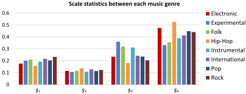
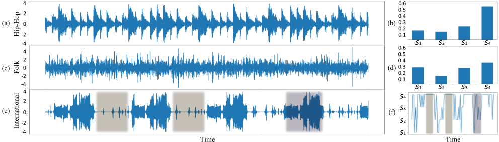
Furthermore, for each genre, we count the weights assigned to each scale, averaging over all the samples and all the time steps t when t MOD sK = 0 (sK = 64). The results are normalized and shown in Fig. 4. Firstly, all the genres prefer to choose larger scales (scale s3 and s4) since the input sequences are so long, and large scale is conducive to modeling the long-term dependence of time series. Meanwhile, there are also significant differences between music of different genres. "Hip-Hop" and "Electronic" prefer to choose the largest scale, compared with the other six. More specifically, Fig. 5 shows three music clips and the corresponding weights assigned to the scales. Music such as "Hip-Hop" is rhythmic and regular, which requires a large scale to model its regularity, thus the weight assigned to scale s4 is large. On the contrary, a smaller scale is sufficient for chaotic music "Folk", since the values of this time series are only related to values within a local window. Therefore, the model would assign similar weights to all four scales. Meanwhile, at each time step t, we record the scale with the largest weight, which is shown in Figure 5(f). The music series in the yellow region has small changes, so there is no need for the model to be updated frequently, and a larger scale would be chosen. On the contrary, series in the purple region varies greatly, thus the choice of scale is more flexible. Similar observations for more examples are shown in the Appendix B. In general, our model better models the multi-scale information of time series and improves the interpretability of the model.
4.4 Ablation Study
Ablation study is conducted on 2 MTS data sets, and the results are shown in Table 4. "LSTM+MSFD(M)" outperforms "LSTM+MSFD(S)" and "LSTM", indicating the importance of multi-scale information. Meanwhile, "LSTM+MSFD(M)"
Time
| Models | FaceDetection | Phoneme |
|---|---|---|
| LSTM | 0.573 | 0.189 |
| CW-LSTM | 0.594 | 0.178 |
| LSTM+MSFD(S) | 0.562 | 0.178 |
| LSTM+MSFD(M) | 0.595 | 0.194 |
| CW-LSTM+TAFM | 0.596 | 0.186 |
| LSTM+MSFD(M)+TAFM | 0.602 | 0.203 |
Table 4: Ablation study on 2 MTS classification data sets. "S" means using single frequency to update different small hidden states, while "M" means using multiple frequencies.
outperforms "CW-LSTM", verifying the effectiveness of MSFD. Finally, the full model (last column) outperforms "LSTM+MSFD(M)" and "CW-LSTM+TAFM", which illustrates the effectiveness of TAFM and MSFD, respectively. The results of other data sets are shown in Appendix C.
4.5 Model Analysis
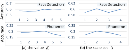
Impact of the value K. To study the influence of the value K (the number of small hidden states), we conduct experiments on 2 MTS classification data sets, FaceDetection and Phoneme. K is set in the range of 1 to 6, and the corresponding scale sets are set to {1}, {1, 2}, {1, 2, 4}, {1, 2, 4, 8}, {1, 2, 4, 8, 16} and {1, 2, 4, 8, 16, 32}, respectively. The results are shown in Figure 6(a). We found that the optimal value K is 4. Increasing K helps to model the multi-scale information of time series, while the hidden size is too small to provide enough features when K is too large.
Impact of the scale set S. The impact of the scale sets is explored and shown in Figure 6(b). 1 to 4 denotes the scale set {1, 2, 3, 4}, {1, 2, 4, 8}, {1, 4, 8, 16} and {1, 4, 16, 64}. The optimal one is {1, 2, 4, 8}. When the range of scales is small, the difference between scales is relatively small, making it hard to learn multi-scale information. When the range of scales is too large, it is hard for a large scale to learn enough information because most time steps are skipped. Other analysis of the model is shown in Appendix D.
5 Conclusion and FutureWork
In this paper, we propose Time-Aware Multi-Scale RNNs (TAMS-RNNs) to capture the multi-scale dynamics of time series adaptively. Instead of using pre-fixed multiple scales, our model disentangles representations of different scales and adaptively selects the most important scale for each sample at each time step. Our experiments demonstrate that TAMSRNNs outperform state-of-the-art methods on different classic time series tasks. Furthermore, the visualization analysis on music genre recognition verifies the effectiveness of the model. In TAMS-RNNs, we use a simple strategy (power of 2) to set the value of each scale, which may not be flexible enough. In future work, we plan to adaptively learn appropriate scale set and apply the model for more other tasks.
Acknowledgements
We thank Prof. Garrison W. Cottrell for his helpful comments and revisions of this paper. The work described in this paper was partially funded by the National Natural Science Foundation of China (Grant Nos. 61502174, 61872148), the Natural Science Foundation of Guangdong Province (Grant Nos. 2017A030313355, 2017A030313358, 2019A1515010768, 2021A1515011496), the Guangzhou Science and Technology Planning Project (Grant Nos. 201704030051, 201902010020), the Key R&D Program of Guangdong Province (Grant No. 2018B010107002), and the Fundamental Research Funds for the Central Universities.
@inproceedings{ijcai2021p315,
  title     = {Time-Aware Multi-Scale RNNs for Time Series Modeling},
  author    = {Chen, Zipeng and Ma, Qianli and Lin, Zhenxi},
  booktitle = {Proceedings of the Thirtieth International Joint Conference on
               Artificial Intelligence, {IJCAI-21}},
  publisher = {International Joint Conferences on Artificial Intelligence Organization},
  editor    = {Zhi-Hua Zhou},
  pages     = {2285--2291},
  year      = {2021},
  month     = {8},
  note      = {Main Track},
  doi       = {10.24963/ijcai.2021/315},
  url       = {https://doi.org/10.24963/ijcai.2021/315},
}
TY - CPAPER TI - Time-Aware Multi-Scale RNNs for Time Series Modeling AU - Chen, Zipeng AU - Ma, Qianli AU - Lin, Zhenxi T2 - Proceedings of the Thirtieth International Joint Conference on Artificial Intelligence, IJCAI-21 PB - International Joint Conferences on Artificial Intelligence Organization PY - 2021 SP - 2285 EP - 2291 DO - 10.24963/ijcai.2021/315 UR - https://doi.org/10.24963/ijcai.2021/315 ER -Copied
Machine-readable versions of this paper, for tools and AI agents:





