
Two Birds with One Stone: Series Saliency for Accurate and Interpretable Multivariate Time Series Forecasting
Proceedings of the Thirtieth International Joint Conference on Artificial Intelligence. Main Track. Pages 2884-2891.
https://doi.org/10.24963/ijcai.2021/397
Keywords
- Machine Learning: Explainable/Interpretable Machine Learning
- Machine Learning: Time-series; Data Streams
Abstract
It is important yet challenging to perform accurate and interpretable time series forecasting. Though deep learning methods can boost forecasting accuracy, they often sacrifice interpretability. In this paper, we present a new scheme of series saliency to boost both accuracy and interpretability. By extracting series images from sliding windows of the time series, we design series saliency as a mixup strategy with a learnable mask between the series images and their perturbed versions. Series saliency is model agnostic and performs as an adaptive data augmentation method for training deep models. Moreover, by slightly changing the objective, we optimize series saliency to find a mask for interpretable forecasting in both feature and time dimensions. Experimental results on several real datasets demonstrate that series saliency is effective to produce accurate time-series forecasting results as well as generate temporal interpretations.
- [Assaf et al., 2019] Roy Assaf, Ioana Giurgiu, Frank Bage- horn, and Anika Schumann. Mtex-cnn: Multivariate time series explanations for predictions with convolutional neu- ral networks. In IEEE International Conference on Data Mining (ICDM), pages 952-957. IEEE, 2019.
- [Baehrens et al., 2010] David Baehrens, Timon Schroeter, Stefan Harmeling, Motoaki Kawanabe, Katja Hansen, and Klaus-Robert Müller. How to explain individual classifi- cation decisions. Journal of Machine Learning Research, 11:1803-1831, 2010.
- [Bahdanau et al., 2014] Dzmitry Bahdanau, Kyunghyun Cho, and Yoshua Bengio. Neural machine translation by jointly learning to align and translate. arXiv:1409.0473, 2014.
- [Box and Jenkins, 1976] George EP Box and Gwilym M Jenkins. Time series analysis, forecasting and control. Holden-Day, 1976.
- [Castelvecchi, 2016] Davide Castelvecchi. Can we open the black box of ai? Nature News, 538(7623):20, 2016.
- [Castro et al., 2009] Javier Castro, Daniel Gómez, and Juan Tejada. Polynomial calculation of the shapley value based on sampling. Computers & Operations Research, 36(5):1726-1730, 2009.
- [Chen et al., 1990] Sheng Chen, Stephen A Billings, and PM Grant. Non-linear system identification using neural networks. International journal of control, 51(6):1191- 1214, 1990.
- [Chung et al., 2014] Junyoung Chung, Caglar Gulcehre, KyungHyun Cho, and Yoshua Bengio. Empirical evalua- tion of gated recurrent neural networks on sequence mod- eling. arXiv:1412.3555, 2014.
- [Dabkowski and Gal, 2017] Piotr Dabkowski and Yarin Gal. Real time image saliency for black box classifiers. In NeurIPS, pages 6967-6976, 2017.
- [Gamboa, 2017] John Cristian Borges Gamboa. Deep learn- ing for time-series analysis. arXiv:1701.01887, 2017.
- [Goodfellow et al., 2016] Ian Goodfellow, Yoshua Bengio, Aaron Courville, and Yoshua Bengio. Deep learning, vol- ume 1. MIT press Cambridge, 2016.
- [Harvey, 1990] Andrew C Harvey. Forecasting, structural time series models and the Kalman filter. Cambridge uni- versity press, 1990.
- [Hochreiter and Schmidhuber, 1997] Sepp Hochreiter and Jürgen Schmidhuber. Long short-term memory. Neural Computation, 9(8):1735-1780, 1997.
- [Hyndman and Athanasopoulos, 2018] Rob J Hyndman and George Athanasopoulos. Forecasting: principles and practice. OTexts, 2018.
- [Ismail et al., 2020] Aya Abdelsalam Ismail, Mohamed Gu- nady, Héctor Corrada Bravo, and Soheil Feizi. Bench- marking deep learning interpretability in time series pre- dictions. arXiv:2010.13924, 2020.
- [Iwana and Uchida, 2020] Brian Kenji Iwana and Seiichi Uchida. An empirical survey of data augmentation for time series classification with neural networks. arXiv preprint arXiv:2007.15951, 2020.
- [Lai et al., 2018] Guokun Lai, Wei-Cheng Chang, Yiming Yang, and Hanxiao Liu. Modeling long-and short-term temporal patterns with deep neural networks. In Inter- national Conference on Information Retrieval, pages 95- 104, 2018.
- [Lundberg and Lee, 2017] Scott M Lundberg and Su-In Lee. A unified approach to interpreting model predictions. In NIPS, pages 4765-4774, 2017.
- [Mitrea et al., 2009] CA Mitrea, CKM Lee, and Z Wu. A comparison between neural networks and traditional fore- casting methods: A case study. International journal of engineering business management, 1:11, 2009.
- [Nussbaumer, 1981] Henri J Nussbaumer. The fast fourier transform. In Fast Fourier Transform and Convolution Al- gorithms, pages 80-111. Springer, 1981.
- [Petersen and Posner, 2012] Steven E Petersen and Michael I Posner. The attention system of the human brain: 20 years after. Annual review of neuroscience, 35:73-89, 2012.
- [Ribeiro et al., 2016] Marco Tulio Ribeiro, Sameer Singh, and Carlos Guestrin. "why should i trust you?" explain- ing the predictions of any classifier. In SIGKDD, pages 1135-1144, 2016.
- [Samek et al., 2019] Wojciech Samek, Grégoire M., Andrea Vedaldi, Lars Kai Hansen, and Klaus-Robert Müller. Ex- plainable AI: interpreting, explaining and visualizing deep learning, volume 11700. Springer Nature, 2019.
- [Serrano and Smith, 2019] Sofia Serrano and Noah A Smith. Is attention interpretable? In Proceedings of the 57th An- nual Meeting of the Association for Computational Lin- guistics, pages 2931-2951, 2019.
- [Shih et al., 2019] Shun-Yao Shih, Fan-Keng Sun, and Hung-yi Lee. Temporal pattern attention for multivari- ate time series forecasting. Machine Learning, 108(8- 9):1421-1441, 2019.
- [Shrikumar et al., 2017] Avanti Shrikumar, Peyton Green- side, and Anshul Kundaje. Learning important features through propagating activation differences. arXiv:1704.02685, 2017.
- [Suresh et al., 2017] Harini Suresh, Nathan Hunt, Alistair Johnson, Leo Anthony Celi, Peter Szolovits, and Marzyeh Ghassemi. Clinical intervention prediction and under- standing using deep networks. arXiv:1705.08498, 2017.
- [Vaswani et al., 2017] Ashish Vaswani, Noam Shazeer, Niki Parmar, Jakob Uszkoreit, Llion Jones, Aidan N Gomez, Lukasz Kaiser, and Illia Polosukhin. Attention is all you need. In NeurIPS, pages 5998-6008, 2017.
- [Zeiler and Fergus, 2014] Matthew D Zeiler and Rob Fergus. Visualizing and understanding convolutional networks. In ECCV, pages 818-833. Springer, 2014.
References were extracted automatically from the PDF and may contain errors.
Full text extracted automatically from the PDF; figures, tables and equations may differ. The PDF is the version of record.
1 Introduction
Time series forecasting is an important task with wide applications. Traditional parametric models often have a shallow architecture (e.g., [Box and Jenkins, 1976; Harvey, 1990]). By adopting some explicit assumptions, such methods are easy-to-interpret, but their predictive capabilities are often limited. Deep architectures have become increasingly popular for time-series [Gamboa, 2017], including recurrent neural networks (RNN), nonlinear autoregressive exogenous neural network (NARX) [Chen et al., 1990], long-short term memory (LSTM) [Hochreiter and Schmidhuber, 1997], gated recurrent unit (GRU) [Chung et al., 2014] and neural attention methods. Though effective in improving forecasting accuracy, deep models are hard to interpret the outputs [Castelvecchi, 2016], which may hinder their applications to high stakes applications (e.g., healthcare) where reliable interpretation is crucial. Though much progress has been made on interpreting deep visual or language models [Samek et al., 2019], it is relatively unexplored to develop both accurate and interpretable methods for multivariate time series forecasting, where the 2D time-feature format imposes new challenges.
∗Contact Author
Existing work often considers either the time or feature domain, or treats them separately via a two-stage method. For example, some attempts have been made to apply the interpretation methods for general neural networks, such as LIME [Ribeiro et al., 2016], DeepLift [Shrikumar et al., 2017] and Shap [Lundberg and Lee, 2017]. They use gradient information to extract feature information for singletime forecasts after the back-propagation training, thereby ignoring the crucial temporal information and insufficient for forecasting interpretation [Mitrea et al., 2009]. Another type of solutions transfers the attention methods from the fields of language or vision [Bahdanau et al., 2014; Vaswani et al., 2017; Assaf et al., 2019; Shih et al., 2019]. However, the attention values for explaining RNNs or CNNs are calculated via the relative importance of the different time steps and there are concerns that they are based on the intermediate feature importance instead of model interpretations [Serrano and Smith, 2019]. More recently, Ismail et al. [Ismail et al., 2020] develop a two-stage saliency approach that decouples the time dimension and feature dimension, thereby may lead to sub-optimal solutions.
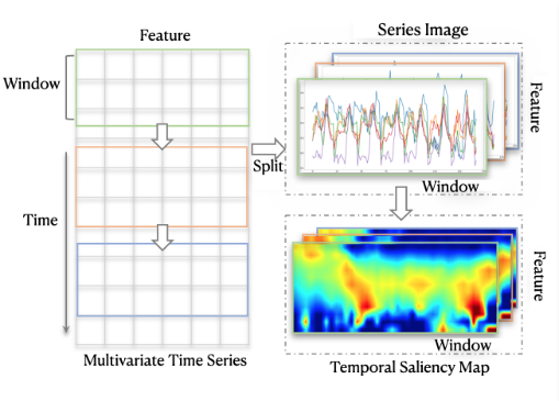
In this work, we present a new strategy of series saliency to boost both forecasting accuracy and interpretability of deep time series models, by considering the time and feature dimensions in a coherent manner. As shown in Fig. 1, we consider multivariate time series as a set of window × feature series images, and design series saliency as a masked mixup between series images and their perturbed versions, where the mask is a learnable matrix. Series saliency is model agnostic and can be used as an effective data augmentation method to boost the accuracy of deep forecasting models, where the augmentation strategy is learnable and adaptive, thereby different from the common augmentation methods (e.g., [Iwana and Uchida, 2020]) that typically apply some pre-fixed operations on a given training set. Furthermore, by simply changing the objective function, we can optimize the series saliency module to find a mask (i.e., heatmap) that identifies important regions for forecasting, thereby boosting interpretability. We present both quantitative and qualitative results on several typical time series datasets, which show that our method achieves better (or comparable) forecasting results and meanwhile provides temporal interpretations for the forecasts.
2 Methods
We now present our method in detail, which consists of a series saliency module and its use in both training and interpretation phases.
2.1 Setup and Notations
As shown in Fig. 1, multivariate time series data are spatiotemporal with two dimensions - time and feature. Formally, we use S to denote a series of observed time series signal:
where st ∈ RD denotes the feature vector with dimension D at time t. For every time step t, we aim to predict the future value st+τ after a given horizon τ. The horizon is chosen according to the forecasting task settings. For example, for the traffic usage, the horizon τ of interest ranges from an hour to a day; while for the stock market data, even a second or minute ahead forecasting can be meaningful for generating returns. Besides forecasting accuracy, we are also interested in interpretation: which features contribute most and which contributes least for the final forecast predictions?
As stated above, traditional statistical methods (e.g., [Box and Jenkins, 1976] and [Harvey, 1990]) are easy to interpret by making some explicit model assumptions that can extract interpretations directly from the learned model parameters, while they are often limited in forecasting accuracy. In contrast, recent progress on deep learning methods leads to superior prediction capabilities [Goodfellow et al., 2016], however, they are hard to interpret since the deep model assumptions are stacked with multiple non-linear activation or blocks.
A key part of an effective model for multivariate time series forecasting would be the capability on handling the information from both time and feature dimensions in a coherent manner. Recent work develops an attention-based scheme [Assaf et al., 2019; Shih et al., 2019], which introduces an attention map to "selectively" combine time-feature information (see Fig. 2 (left)), with the primary focus on interpretation. However, as pointed out in [Ismail et al., 2020], the attention-based methods can be insufficient for interpreting multivariate time-series data. We develop a new scheme of series saliency, which is model-agnostic and can boost both forecasting accuracy and interpretation, as detailed below.
2.2 Series Saliency
We develop series saliency by drawing inspirations from the saliency maps [Dabkowski and Gal, 2017] in computer vision. However, unlike previous work on saliency maps that mainly focuses on interpetability of deep models, series saliency is beneficial for improving both forecasting accurarcy and interpretation for time-series data.
Specifically, to consider the time-feature information jointly, we first represent the multivariate time series as a set of 2D series images. As shown in Fig. 1, each series image corresponds to a part of the multivariate time series within a given time window. Formally, let T be the window size. We simply set the value of T for various datasets with 2 periodic patterns (e.g., p = 48 for hourly electricity consumption). A series image is represented as a matrix X ∈ RD×T , of which each row corresponds to one feature dimension in the multivariate time series. Then, we follow the perturbation strategy in the smallest destroying region (SDR) principle [Dabkowski and Gal, 2017] to design the series saliency scheme. We define a reference series image ˆX by adding noise or Gaussian blur on each element of the original series image X:
where ϵσ1 ∼ N(µ, σ2 1 ) is a Gaussian noise and gσ2 is a Gaussian blur kernel on element xt,i with the maximum isotropic standard deviation σ2.
In time series data, each series can be composed of three parts - trend, seasonality and residual [Hyndman and Athanasopoulos, 2018]. As shown in [Hyndman and Athanasopoulos, 2018], blurring is helpful to extract the trend information of a time series, and adding some noise can enhance the local information. When the amount of injected noise or blurring is small, the reference series images can be treated as data augmentation in the time domain [Iwana and Uchida, 2020] to learn deep models. However, if the noise (or blurring) is not set properly (e.g., too large), the noise (or blurring) will introduce irregular roughness to cover the original series, making it difficult for DNNs to learn temporal patterns in reference data.
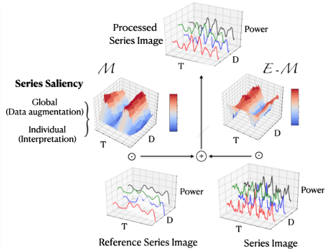
To relieve the sensitivity over noise (or blurring), the series saliency module further introduces a learnable mask M ∈ [0, 1]D×T and selectively combines the reference series image and the original one:
where E is the matrix with all elements be the unit one. As illustrated in Fig. 1, in such a design, the series saliency module can generate data (i.e., ˜X) that cover the unexplored input space while maintaining the important characteristics of the original series image (i.e., X). As we shall see, series saliency is an effective data augmentation strategy for training deep models and it is learnable.
Besides augmenting the data for improving training, series saliency can also be used for interpretation by simply changing the objective to be optimized. We defer the details to Section 2.4 after presenting the training procedure.
2.3 Training with Series Saliency
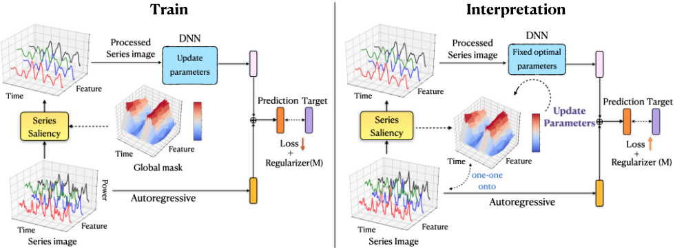
With the series saliency module, we now present the entire model architecture and its training details. One essential problem in deep learning models is that the scale of the outputs is not sensitive to the scale of inputs. In specific real time series datasets, the scale of input data often changes in a non-periodic manner, which can significantly lower the forecasting accuracy of deep learning models. We propose to decompose the final prediction into a linear part, which primarily focuses on the local scaling issue, plus a non-linear part containing complex temporal patterns. Fig. 2 (left) shows the dual-path architecture - a nonlinear deep learning (DL) module and a linear auto-regressive (AR) module.
The original series images X are converted to the processed versions ˜X by our proposed module, and then ˜X are fed into the DL module to obtain y(r) . Here, the DL module can be any time series network, e.g., convolution neural networks, recurrent neural networks, Long short-term memory (LSTM) [Hochreiter and Schmidhuber, 1997], long- and short-term temporal pattern neural network (LSTNet) [Lai et al., 2018] and Self-Attention encoder [Vaswani et al., 2017] (see experiments for details). For the linear part, we choose an auto-regressive model and denote its result as y(o) :
where p is the order of the AR model, Wk ∈ RD and b ∈ R are its coefficients. p can be determined for various datasets with periodic patterns (e.g., p = 24 for the hourly electricity consumption). In our experiments, we empirically searched a good p through validation. The final forecasting is obtained by combining the outputs of both DL and AR:
Let N be the number of series images in the training set and φ = {θ,W, b} denote all the unknown parameters. For notation simplicity, we will use yi to denote the ground-truth forecasting result of Xi at a particular horizon. We adopt stochastic gradient descent (SGD) to jointly optimize over φ and M. Specifically, at each iteration, we draw a mini-batch B = {(Xi, yi)}ni=1 with size n. Our loss function ℓ(φ,M) consists of two parts. First, for each (Xi, yi) ∈ B, we follow the diagram in Fig. 2 to get the prediction ˆ yi (a function of both φ and M) via Eq. (5), and accumulate the squared error
‖ˆ yi - yi‖2 into the loss ℓ(φ,M). Second, to fully leverage the training set, we also send the original series image Xi into both the DNN and AR model (i.e., bypassing the series saliency module in Fig. 2 to get another prediction ˆ y′i (a function of φ only) via Eq. (5), and accumulate the squared error ‖ˆ y′i - yi‖2 into the loss ℓ(φ,M). Our overall training objective is to minimize a regularized version of loss ℓ(φ,M):
where ℓm(M) and ℓr(M) are regularization terms on the mask M, λ1 and λ2 are the corresponding coefficients.
The effect of the regularizer ℓm(M) is to control the amount of perturbation. As stated before, if M is close to E, the reference series image will dominate and may degenerate the performance. To discourage such degenerating case, we choose the common 2-norm, i.e., ℓm(M) = ‖M‖2.
The design of ℓr(M) is a bit more subtle. Note that a key difference exists between our series images and the natural images in computer vision - the rows (i.e., features) of series images are permutable without affecting the content, while switching the rows of a nature image would destroy its semantic meaning. In our case, we would expect the feature importance matrix M to be row-wisely orthogonal. Therefore, we define the regularizer term ℓr(M):
where I is the identity matrix and ||·||F is the Frobenius norm. Such orthogonality is beneficial for interpretation, and can boost the training as well (see ablation study in Section 3.2).
With the overall objective L1, we use back-propagation to calculate its gradient and apply SGD to update (φ,M). We would like to highlight a key difference from the traditional data augmentation [Iwana and Uchida, 2020]. Unlike the traditional methods, which typically augment the data for once with some pre-fixed strategies (e.g., perturbation with a fixed noise), our augmentation strategy is adaptive by iteratively updating the mask M of the series saliency module. Such a scheme makes the model to better focus on informative parts that are good for forecasting, as we shall see in experiments.
2.4 Interpretation with Series Saliency
Now, we show that with the series saliency module, we can easily derive an interpretation strategy for forecasting.
Let X∗ be the a series image in the testing set with groundtruth forecasting y∗ at a particular horizon τ. Let φ∗ denote the optimal parameters of the DNN and AR models after training. We follow the diagram in Fig. 2 to get the prediction ˆ y∗ (a function of M) via Eq. (5), and calculate the squared error ‖ˆ y∗ - y∗ ‖2 . The goal of interpretation is to find the most salient evidence that influences the model performance measured by square error. In series saliency, the most salient feature regions are found by identifying the highly representative mask, which summarizes compactly the effect of deleting feature regions, either setting values to zeros or Gaussian noise, to explain the behaviour of the DL part. For the AR part, the weights are easy-to-interpret because of its linearity [Hyndman and Athanasopoulos, 2018]. On the other hand, the AR part mainly assists DL models to address the local scaling issue, so it is not essential to focus on the explanation of the AR
part. Formally, we formulate interpretation as minimizing the following objective:
where ℓm(M) and ℓr(M) are the same regularization terms as in training. Then, we use back-propagation to calculate the gradient of L2 and apply SGD to update M only. After convergence, the optimal M provides an interpretation of important features for forecasting on instance X∗ .
3 Experiments
We now present experimental results by comparing the performance of four widely-used deep learning models with and without the proposed series saliency module on various datasets. We also give an ablation study on the mask and AR model components. Then we show extensive qualitative results on how saliency heatmaps interpret the forecasts.
3.1 Experimental Setting
(1) Datasets: We use three time series datasets electricity, Air-quality, Industry data The three datasets are representative (from difficult to easy). (2) Metrics: We use two evaluation metrics, namely relative squared error (RSE) and empirical correlation coefficient (CORR). For RSE, lower values are better, while for CORR higher values are better. The datasets and the metrics have been widely used in many papers about time series forecasting (e.g., LSTNet, TPA-LSTM) [Lai et al., 2018; Shih et al., 2019]. (3) Deep Learning Module: We use four state-of-the-art architectures for comparison (i.e., CNN, GRU+Attention, LSTNet and Self-Attention encoder). These four deep learning models achieve superior forecasting performance and in the following results they are used as the deep learning module to get interpreted by the proposed series saliency method.
3.2 Results on Forecasting
Table 1 presents the CORR values of various methods on the three datasets with different forecasting horizons. We can see that using the series saliency module can boost the forecasting accuracy of various deep models on the Air quality dataset, especially when the forecasting horizon is large. This is because the model complexity increases with the horizon, and data augmentation may help explore more useful temporal information. We also observe that among all the deep architectures in comparison, the Self-Attention encoder with the series saliency gives the best performance in most settings, mainly because of the powerful representation capability of the transformer encoder model. Therefore, in the sequel, we will use the Self-Attention encoder as the main architecture to do further analysis.
Ablation Study
We now present an ablation study to demonstrate the effectiveness of our design components, including regularization terms and and the auto-regressive path in our architecture.
First, we examine how the auto-regressive module helps on the forecasting when series saliency (i.e., data augmentation) is used. We compare the following variants:
| Methods | τ = 3 | Air Quality τ = 6 | τ = 12 | τ = 3 | Industry τ = 6 | τ = 12 | τ = 3 | Electricity τ = 6 | τ = 12 |
|---|---|---|---|---|---|---|---|---|---|
| CNN | 0.775 ± 0.003 | 0.701 ± 0.001 | 0.636 ± 0.001 | 0.919 ± 0.022 | 0.909 ± 0.019 | 0.841 ± 0.008 | 0.883 ± 0.004 | 0.871 ± 0.002 | 0.866 ± 0.004 |
| GRU | 0.804 ± 0.003 | 0.712 ± 0.002 | 0.639 ± 0.003 | 0.953 ± 0.003 | 0.936 ± 0.013 | 0.904 ± 0.011 | 0.878 ± 0.001 | 0.877 ± 0.003 | 0.867 ± 0.002 |
| LSTNet | 0.777 ± 0.001 | 0.708 ± 0.004 | 0.624 ± 0.004 | 0.949 ± 0.004 | 0.934 ± 0.003 | 0.876 ± 0.011 | 0.922 ± 0.004 | 0.913 ± 0.002 | 0.906 ± 0.002 |
| SA | 0.813 ± 0.002 | 0.722 ± 0.003 | 0.643 ± 0.003 | 0.961 ± 0.002 | 0.942 ± 0.005 | 0.905 ± 0.009 | 0.919 ± 0.007 | 0.907 ± 0.001 | 0.902 ± 0.003 |
| CNNw/ SS | 0.779 ± 0.005 | 0.723 ± 0.009 | 0.641 ± 0.007 | 0.941 ± 0.006 | 0.927 ± 0.004 | 0.881 ± 0.001 | 0.898 ± 0.004 | 0.893 ± 0.002 | 0.892 ± 0.007 |
| GRUw/ SS | 0.809 ± 0.003 | 0.716 ± 0.012 | 0.649 ± 0.003 | 0.955 ± 0.001 | 0.935 ± 0.002 | 0.912 ± 0.003 | 0.905 ± 0.004 | 0.889 ± 0.008 | 0.878 ± 0.003 |
| LSTNet w/ SS | 0.794 ± 0.008 | 0.724 ± 0.002 | 0.641 ± 0.003 | 0.959 ± 0.004 | 0.938 ± 0.001 | 0.901 ± 0.002 | 0.928 ± 0.003 | 0.918 ± 0.003 | 0.907 ± 0.001 |
| SAw/ SS | 0.819 ± 0.003 | 0.732 ± 0.009 | 0.658 ± 0.001 | 0.965 ± 0.003 | 0.955 ± 0.016 | 0.916 ± 0.004 | 0.923 ± 0.003 | 0.915 ± 0.001 | 0.911 ± 0.002 |
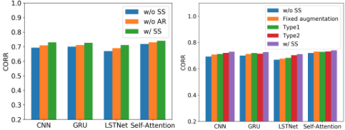
- w/ SS: The model in Fig. 2 with series saliency (SS).
- w/o SS: The model in Fig. 2, but without series saliency;
- w/o AR: The model in Fig. 2 with series saliency, but without the auto-regressive component.
Fig. 3 (left) shows the results. We do not use any perturbation in w/o SS. We can see that both the series saliency (i.e., adaptive data augmentation) and the auto-regressive modules are helpful to boost the performance - dropping either one would lead to degenerated performance.
Second, we do a finer investigation on the effects of the regularization terms in learning the series saliency module during training. We compare the following variants:
- w/o SS: The model in Fig. 2, but without the series saliency module (i.e., no data augmentation);
- Fixed augmentation: Augment the series images for once with some prefixed strategies (perturbation with a fixed noise) [Iwana and Uchida, 2020].
- Type1: The entire model in Fig. 2 trained by minimizing the loss only (i.e., without ℓr and ℓm).
- Type2: The entire model in Fig. 2 trained by minimizing the loss with ℓm regularizer (i.e., without ℓr).
- w/ SS: The entire model in Fig. 2 trained with both ℓr and ℓm regularizers as in Eq. (6).
Fig. 3 (right) shows the results. Again, we can see that series saliency can boost the forecasting results (i.e., higher CORR). Also, being an adaptive strategy, series saliency is more effective for training deep models than the pre-fixed data augmentation method [Iwana and Uchida, 2020]. The regularizer term ℓm has little effect on improving the model performance, while ℓr is much more influential. By considering the decouple of feature importance in time series help the neural networks understand time series data accurately.
3.3 Results on Interpretation
We present both qualitative and quantitative results.
Qualitative Analysis
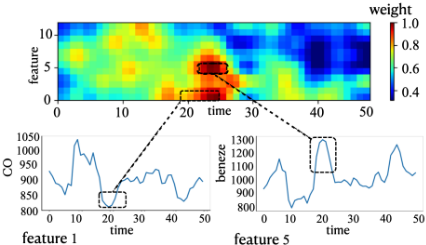
We apply the series saliency methods with the Self-Attention encoder model on the air quality dataset. Fig. 5 visualizes the learned mask component when forecasting the selected future value with horizon τ = 6. As the color bar shows, from blue to red means that the features become more and more important. We can see that the features from time interval [20, 30] have the largest saliency, which corresponds to the extreme low value in feature 1 representing the concentration of CO and high value in feature 5 representing the concentration of benzene.
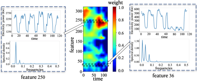
We also visualize the correspondence between saliency mask, the original time series data and the data frequencies on the electricity dataset. Fig. 4 shows the results. We can see that the data of channel 250 has the high value of the saliency mask and reflects a periodic structure (top left in Fig. 4). In contrast, the data of channel 36 has the low value of the saliency mask and reflects a relatively acylic structure (top right in Fig. 4). Furthermore, to prove the periodicity of our selected a channels, we map the corresponding feature to a frequency domain by a fast fourier transform procedure (FFT) [Nussbaumer, 1981] and show the frequency result below the data of the two channels.
Quantitative Comparison
Finally, similar as in [Ismail et al., 2020], we present a quantitative metric to evaluate the interpretability for time series forecasting and compare with various baselines.
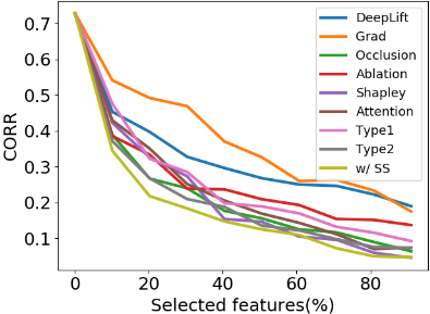
Specifically, for each testing example X, we use a given interpretation method to generate the feature importance map, and select the top k features. Then, we add the random Gaussian noise on the selected features, and feed the perturbed version into the pretrained model for forecasting. Given a testing set, we calculate the corresponding CORR value. We change the value of k = [10%, ..., 90%], and obtain the decreasing CORR curve with different k (i.e., different perturbation levels). Finally, we calculate the area under the CORR curve as the quantitative metric and denote it by AUCORR. The lower AUCORR values mean that we select the more important features ßand the interpretation method is more effective.
We compare with a wide range of baselines including Grad [Baehrens et al., 2010], DeepLift [Shrikumar et al., 2017], feature ablation [Suresh et al., 2017], Occlusion [Zeiler and Fergus, 2014], Shapely sampling [Castro et al., 2009] and attention [Petersen and Posner, 2012]. Also, to examine the effect of regularizers in interpretation, we consider the following variants of our method:
- w/ SS: The model in Fig. 2 interpreted with both ℓr and ℓm regularizers as in Eq. (8);
- Type1: The model in Fig. 2 interpreted by minimizing the loss L2 only (i.e., without ℓr and ℓm);
- Type2: The model in Fig. 2 interpreted by minimizing the loss L2 with ℓr regularizer (i.e., without ℓm).
Table 2 and Fig. 6 show the results. We can see that the series saliency map by our method can obtain the best quantitative interpretation results compared to those by other interpretation results (e.g., DeepLift and attention). Moreover, the two regularization terms ℓm and ℓr are useful to improve the interpretation results. In general, although we can't guarantee any selected future values will have the representative interpretation in qualitative analysis (e.g., Fig. 5), the performance of our method is quantitatively superior to other competitors.
4 Conclusions
We present a novel scheme of series saliency to boost both accuracy and interpretability for multivariate time series forecasting. By extracting series images from sliding windows of the time series, we design series saliency as a mixup approach with a learnable mask defined on the series images and their perturbed versions. Series saliency acts as an adaptive data augmentation method for training deep models, and meanwhile by slightly changing the objective, it can be optimized to find a mask for interpretable forecasting in both feature and time dimensions. Experimental results show the superiority of series saliency over various baselines.
Acknowledgements
This work was supported by the National Key Research and Development Program of China ( No. 2017YFA0700904,No.2020AAA0104304), NSFC Projects (Nos. 61620106010, 62076147, U19A2081, U19B2034, U1811461), Beijing Academy of Artificial Intelligence (BAAI), Tsinghua-Huawei Joint Research Program, a grant from Tsinghua Institute for Guo Qiang, Tiangong Institute for Intelligent Computing, and the NVIDIA NVAIL Program with GPU/DGX Acceleration.
| Methods | Industry | Air Quality | Electricity |
|---|---|---|---|
| Grad | 0.214 ± 0.007 | 0.297 ± 0.007 | 0.199 ± 0.008 |
| DeepLift | 0.211 ± 0.008 | 0.241 ± 0.006 | 0.174 ± 0.003 |
| Ablation | 0.204 ± 0.008 | 0.225 ± 0.006 | 0.213 ± 0.009 |
| Occlusion | 0.124 ± 0.004 | 0.221 ± 0.011 | 0.142 ± 0.005 |
| Shapley | 0.145 ± 0.006 | 0.211 ± 0.010 | 0.171 ± 0.005 |
| Attention | 0.141 ± 0.007 | 0.203 ± 0.007 | 0.139 ± 0.003 |
| Type1 | 0.131 ± 0.005 | 0.205 ± 0.008 | 0.143 ± 0.004 |
| Type2 | 0.122 ± 0.002 | 0.201 ± 0.005 | 0.135 ± 0.001 |
| w/ SS | 0.117 ± 0.002 | 0.192 ± 0.003 | 0.131 ± 0.002 |
@inproceedings{ijcai2021p397,
  title     = {Two Birds with One Stone: Series Saliency for Accurate and Interpretable Multivariate Time Series Forecasting},
  author    = {Pan, Qingyi and Hu, Wenbo and Chen, Ning},
  booktitle = {Proceedings of the Thirtieth International Joint Conference on
               Artificial Intelligence, {IJCAI-21}},
  publisher = {International Joint Conferences on Artificial Intelligence Organization},
  editor    = {Zhi-Hua Zhou},
  pages     = {2884--2891},
  year      = {2021},
  month     = {8},
  note      = {Main Track},
  doi       = {10.24963/ijcai.2021/397},
  url       = {https://doi.org/10.24963/ijcai.2021/397},
}
TY - CPAPER TI - Two Birds with One Stone: Series Saliency for Accurate and Interpretable Multivariate Time Series Forecasting AU - Pan, Qingyi AU - Hu, Wenbo AU - Chen, Ning T2 - Proceedings of the Thirtieth International Joint Conference on Artificial Intelligence, IJCAI-21 PB - International Joint Conferences on Artificial Intelligence Organization PY - 2021 SP - 2884 EP - 2891 DO - 10.24963/ijcai.2021/397 UR - https://doi.org/10.24963/ijcai.2021/397 ER -Copied
Machine-readable versions of this paper, for tools and AI agents:





