
Towards Reducing Biases in Combining Multiple Experts Online
Proceedings of the Thirtieth International Joint Conference on Artificial Intelligence. Main Track. Pages 3024-3030.
https://doi.org/10.24963/ijcai.2021/416
© 2021 International Joint Conferences on Artificial Intelligence
Keywords
- Machine Learning: Online Learning
- AI Ethics, Trust, Fairness: Fairness
Abstract
In many real life situations, including job and loan applications, gatekeepers must make justified and fair real-time decisions about a person’s fitness for a particular opportunity. In this paper, we aim to accomplish approximate group fairness in an online stochastic decision-making process, where the fairness metric we consider is equalized odds. Our work follows from the classical learning-from-experts scheme, assuming a finite set of classifiers (human experts, rules, options, etc) that cannot be modified. We run separate instances of the algorithm for each label class as well as sensitive groups, where the probability of choosing each instance is optimized for both fairness and regret. Our theoretical results show that approximately equalized odds can be achieved without sacrificing much regret. We also demonstrate the performance of the algorithm on real data sets commonly used by the fairness community.
- [Angwin et al., 2016] Julia Angwin, Jeff Larson, Surya Mattu, and Lauren Kirchner. Machine bias. ProPublica, May 23rd, 2016.
- [Arora et al., 2012] Sanjeev Arora, Elad Hazan, and Satyen Kale. The multiplicative weights update method: a meta- algorithm and applications. Theory of Computing, 8:121- 164, 2012.
- [Bechavod et al., 2019] Yahav Bechavod, Katrina Ligett, Aaron Roth, Bo Waggoner, and Steven Z. Wu. Equal op- portunity in online classification with partial feedback. In NeurIPS, 32, pages 8972-8982. 2019.
- [Blum et al., 2018] Avrim Blum, Suriya Gunasekar, Thodoris Lykouris, and Nati Srebro. On preserving non-discrimination when combining expert advice. In NeurIPS, 31, pages 8376-8387. 2018.
- [Celis et al., 2019] L. Elisa Celis, Lingxiao Huang, Vijay Keswani, and Nisheeth K. Vishnoi. Classification with fairness constraints: A meta-algorithm with provable guar- antees. In Proc. of the Conf. on Fairness, Accountability, and Transparency, pages 319-328, 2019.
- [Chouldechova, 2017] Alexandra Chouldechova. Fair pre- diction with disparate impact: A study of bias in recidi- vism prediction instruments. Big data, 5 2:153-163, 2017.
- [Corbett-Davies et al., 2017] Sam Corbett-Davies, Emma Pierson, Avi Feller, Sharad Goel, and Aziz Huq. Algo- rithmic decision making and the cost of fairness. In KDD, 2017.
- [Donini et al., 2018] Michele Donini, Luca Oneto, Shai Ben- David, John S Shawe-Taylor, and Massimiliano Pontil. Empirical risk minimization under fairness constraints. In NeurIPS, 31, pages 2791-2801, 2018.
- [Dwork et al., 2012] Cynthia Dwork, Moritz Hardt, Toniann Pitassi, Omer Reingold, and Richard Zemel. Fairness through awareness. In Proc. of the 3rd Innovations in The- oretical Computer Science Confe., ITCS '12, pages 214- 226, 2012.
- [Gillen et al., 2018] Stephen Gillen, Christopher Jung, Michael Kearns, and Aaron Roth. Online learning with an unknown fairness metric. In NeurIPS, 31, pages 2600-2609. 2018.
- [Hardt et al., 2016] Moritz Hardt, Eric Price, and Nathan Srebro. Equality of opportunity in supervised learning. In NeurIPS, 29, pp. 3315-3323, 2016.
- [Joseph et al., 2016] Matthew Joseph, Michael Kearns, Jamie H. Morgenstern, and Aaron Roth. Fairness in learning: Classic and contextual bandits. In NeurIPS, pages 325-333, 2016.
- [Kleinberg et al., 2017] Jon Kleinberg, Sendhil Mul- lainathan, and Manish Raghavan. Inherent trade-offs in the fair determination of risk scores. Innovations in Theoretical Computer Science, 2017.
- [Liu et al., 2017] Yang Liu, Goran Radanovic, Christos Dimitrakakis, Debmalya Mandal, and David C. Parkes. Calibrated fairness in bandits. In Proceedings of the 4th Workshop on Fairness, Accountability, and Transparency in Machine Learning (Fat/ML 2017), 2017.
- [Zafar et al., 2015] Muhammad Bilal Zafar, Isabel Valera, Manuel Gomez Rodriguez, and Krishna P Gummadi. Fair- ness constraints: Mechanisms for fair classification. arXiv preprint arXiv:1507.05259, 2015.
- [Zafar et al., 2017] Muhammad Bilal Zafar, Isabel Valera, Manuel Gomez-Rodriguez, and Krishna P. Gummadi. Fairness beyond disparate treatment and disparate impact: Learning classification without disparate mistreatment. In Proc. of the 26th Int. Conf. on World Wide Web, pages 1171-1180, 2017.
References were extracted automatically from the PDF and may contain errors.
Full text extracted automatically from the PDF; figures, tables and equations may differ. The PDF is the version of record.
1 Introduction
In the near future, machine learning models are expected to aid decision-making in a variety of fields. Recently, however, concerns have arisen that machine learning models may accentuate preexisting human biases and data imbalances, affecting decision-making and leading to unfair outcomes in areas including policing [Angwin et al., 2016], college admissions, and loan approvals.
The machine learning community has responded to this critique by designing strategies to train a fairer classifier [Zafar et al., 2015][Donini et al., 2018], yet this is not always a feasible solution. There are many situations in which decisions are not made by a trainable classifier, but instead by human experts or black-box models. A better solution, then, would be an online policy balancing accuracy and fairness without considering individual experts' technical underpinnings. Indeed, ensuring fairness via a mathematical framework would ideally not only prevent prejudice within algorithms, but help quantitatively overcome human biases as well.
Here another important question arises: what, exactly, is fairness? In general, the machine-learning community agrees to aim for statistical parity - the equalization of some measure of errors across protected groups. These measures include equal opportunity [Hardt et al., 2016], equalized odds (disparate mistreatment) [Zafar et al., 2017][Hardt et al., 2016] and predictive parity [Celis et al., 2019]. In this paper, we focus on achieving equalized odds and emphasizing that all error types should be addressed, i.e., equalized across groups, rather than equalizing a combined measure. Previous online strategies for fairness do not solve for equalized odds [Blum et al., 2018][Bechavod et al., 2019].
Finally, in many cases, people will strategically react to a decision-making process, leaving models to face shifting distributions. For instance, if a particular job has historically employed more males than females, the position might attract more males to apply, worsening the bias in the distribution. In this situation, having fair base models and a static combining strategy is not enough to overcome bias. Even without access to the base models, an online algorithm must be adaptive over time and maintain equalized odds.
Thus this paper focuses on: an online setting where we have protected underrepresented groups; each individual is randomly sampled i.i.d. from a potentially biased and shifting distribution across groups and labels; and a finite set of classifiers (or experts) that have already been trained where we only have access to their decisions. The goal is to design a randomized algorithm that combines these experts such that the violation of fairness of the resulting "combined expert" can be upper bounded, which further allows us to achieve an optimal balance between fairness and regret.
In this paper we make the following contributions. We propose a randomized algorithm that (i) works in online stochastic settings (individuals sampled from i.i.d. distribution), (ii) has a provable asymptotic upper bound on regret and equalized odds, (iii) the upper bound is minimized to achieve the desired balance between equalized positive rate, equalized negative rate and regret. These give the name GFORCE (Group-Fair, Optimal, Randomized Combination of Experts). Finally, we demonstrate its performance on datasets commonly used by the fairness community, and on synthetic datasets to test its performance under extreme scenarios.
2 RelatedWork
There are two broad definitions for fairness: individual fairness and group fairness. Individual fairness builds upon "treating similar individuals similarly" [Dwork et al., 2012].
On the other hand, group fairness is achieved by balancing certain statistical metrics approximately across different demographic groups (such as groups divided by gender, race, etc). Equalized odds [Zafar et al., 2017] [Hardt et al., 2016], a.k.a. disparate mistreatment, requires that no error type appears disproportionately for any one or more groups. A weaker notion of equalized odds is equal opportunity, which aims to achieve equal false positive rates [Hardt et al., 2016]. equalized odds can be achieved by adding in additional constraints when optimizing the objective function [Zafar et al., 2017], or by enforcing an optimal threshold for a predictor during post-processing [Hardt et al., 2016]. However, recent work shows that it is impossible to achieve equalized odds [Chouldechova, 2017; Kleinberg et al., 2017] simultaneously with other notions of fairness such as calibration, which requires that outcomes are independent of protected attributes conditional on the estimates from predictors. In this paper we consider equalized odds as a fairness metric, but the method can be developed to optimize for other fairness metrics too. It is also generally accepted that there is often a trade-off between predictive accuracy and fairness [Corbett-Davies et al., 2017].
At the same time, there has been recent interest in studying fairness in an online setting, particularly the bandit setting where the goal is to fairly select from a set of individuals at each round. [Joseph et al., 2016] studies the contextual bandit setting with unknown reward functions. [Gillen et al., 2018] considers a problem where the specific individual fairness metric is unknown. [Liu et al., 2017] considers satisfying calibrated fairness in a bandit setting. On the group fairness side, [Bechavod et al., 2019] tries to enforce the equalized opportunity constraint at every round under a partial feedback setting, where only true labels of positively classified instances are observed. [Blum et al., 2018], specifically shows that it is impossible to achieve equalized odds under an adversarial setting when an adaptive adversary can choose which individual to arrive. Our paper considers a more realistic stochastic setting, and proposes an algorithm can achieve approximate equalized odds with a slight increase in regret.
3 Background
In this section, we introduce our setting and the notations we use throughout this papers. We also provide background on the multiplicative weights algorithm and evaluation metrics.
3.1 Settings and Preliminaries
We assume access to a set of black-box classifiers F = {f1, . . . , fd}. While many fairness solutions attempt to optimize a classifier, our goal is to produce fair and accurate predictions by combining the classifiers according to their past performances. In online settings, an algorithm runs through rounds t = 1, . . . , T . At each round t:
- A single example (xt , zt ) ∈ Rn arrives, where xt ∈ X is a vector of unprotected attributes and zt ∈ Z is a protected or sensitive attribute.
- One classifier f t ∈ F is randomly selected to estimate ˆ yt = f t (xt , zt ), the label for the input example.
- The true label yt is revealed after the prediction.
Notations and Assumptions
In this paper we consider binary classification problems, with a positive and a negative class, i.e., y ∈ {+,-}. For the sake of notation, we assume the whole data set can be divided in two population groups A and B according to the sensitive attribute; i.e. z ∈ {A,B}, though our approach can be easily extended to multiple groups. We denote the probability an example coming from group z as pz ; and define the base rates for outcomes in group z as µz,+ = P(y = +|z). Superscript t denotes the time index or round t; for instance yt is the true class of the example given in round t. Superscript ∗ denotes optimality; for instance f ∗ (z, y) represents the best classifier on group z with label y. Superscript T denotes the matrix transpose only when it is on a vector. Letter ℓ denotes a loss function.
Throughout the paper it is often necessary to refer to a classifier f, a group z, the true label y, or a combination of these. We indicate such a combination with a list of subscripts; e.g. wf,z is the multiplicative weight associated to a given classifier f, specific to samples from group z, and ℓf,z,y represents the loss specific to samples from group z and with true label y. These subscripts are replaced with a specific value when necessary. For instance ℓf,z,- specifies that all the samples considered are negative. A lack of subscripts represents the generic variable.
3.2 EvaluationMetrics
A frequent performance metric in online learning is Regret, which compares the performance of the algorithm to that of the best fixed expert in hindsight.
The typical goal of online learning algorithm is to achieve sub-linear regret over T rounds; i.e. lim T→∞ Regret(T )/T = 0. In addition, we try to make the algorithm fair to each sensitive group by considering equalized odds :
Definition 3.1 (Equalized FPR and FNR). Let ˆ y be the estimated outcome from a binary classifier when it receives an instance with protected attributes z and ground truth y.
be the False Positive Rate (FPR) and the False Negative Rate (FNR) for group z. A classifier satisfies Equalized FPR (FNR) on group A and B if FPRA = FPRB (FNRA = FNRB).
Definition 3.2 (Equalized odds). A classifier exhibits equalized odds if it achieves both an equalized FPR and an equalized FNR.
In other words, equalized odds implies that the outcome of the classifier is independent of the protected attributes, given the true class.
Definition 3.3 (Equalized Error Rates). A classifier satisfies equalized error rates (EER) on group A and B if
Definition 3.4 (ϵ-fairness). An algorithm satisfies ϵ-fairness if:
|FPRA -FPRB| ≤ ϵ and |FNRA -FNRB| ≤ ϵ.Thus, a measure of how an algorithm performs in terms of equalized odds is given by: |FPRA -FPRB| and |FNRA - FNRB|, which are sometimes referred throughout the paper as equalized FPR or equalized FNR for simplicity.
3.3 MultiplicativeWeights Algorithm
The Multiplicative Weights (MW) is a well-known algorithm for achieving no regret by combining decisions from multiple experts. The main idea is that the decision maker maintains weights on the experts based on their performances up to the current round, and the algorithm selects an expert according to these weights.
Theorem 1. Assume that the loss ℓtf is bounded in [0,1] and η < 12 . Let ℓtf ∗ be the loss of the best expert after t rounds, then we have:
where πt is the probability mass function (PMF) for selecting the set of classifiers at each round.
This powerful theorem [Arora et al., 2012] shows that the expected cumulative loss achieved by the MW algorithm is upper bounded by the cumulative loss of the best fixed expert in hindsight asymptotically. In other words, the MW algorithm achieves sub-linear regret.
GroupAware Algorithm. [Blum et al., 2018] proposed a GroupAware version of the MW algorithm to achieve equalized error rates (EER) across sensitive groups in an adversarial setting. They showed that to attain EER it is necessary to run separate instances of the original MW algorithm on each sensitive group. One drawback of the GroupAware algorithm is that it only bounds the performance of the overall error for each sensitive group, without any guarantee on the number of false positives and false negatives within each group. In the worst case, GroupAware could have 100% FPR on one sensitive group and 0% FPR on the other, which leads to a severe violation of equalized odds.
4 G-FORCE Algorithm
We argue that it is necessary to run MW instance on a more granular level, in order to satisfy equalized odds. Specifically, it is necessary to keep different instances of the algorithm for each group as well as for each label.
We propose a novel randomized MW algorithm that utilizes not only sensitive groups but also their labels, and show that it is possible to find bounds on the violation of equalized odds. Moreover, the bounds can be further optimized by cleverly coordinating between the instances. For the sake of clarity, the rest of the paper we consider binary classification with two sensitive groups, though the algorithm can be easily extended to multi-group and multi-class problems.
4.1 G-FORCEMechanism
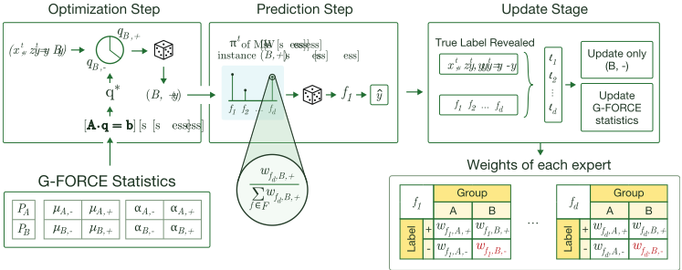
G-FORCE keeps separate MW instances for each possible 2-tuple (z, y) with z ∈ {A,B} and y ∈ {+,-}. Throughout the paper, we use tuple (z, y) to refer to a MW instance trained with group z and label y. Each MW instance associates a weight to a classifier f for group z and label y; e.g. the weight of classifier f for group A and negative label examples is denoted as wf,A,-. The mechanism of G-FORCE is explained in Figure 1. At each round, G-FORCE takes in an example (x, z). G-FORCE works in three steps: optimization step, prediction step and the update step.
Optimization Step. G-FORCE first selects an appropriate MW instance to use. While group z is known, at this point G-FORCE doesn't know the label yet (which is exactly the target to predict) and has to choose between instance (z,+) and instance (z,-). G-FORCE constructs a meta probability, which we refer to as the blind selection rule to select between the two instances, where qz,+ and qz,- are the probability of selecting (z, +), and (z, -) respectively. In the case G-FORCE selects the wrong instance (for example, true label is - but (z,+) is selected), we refer to the additional losses as Cross-Instance Cost αz,+ (formal definition in next section). This meta probability allows us to explicitly construct a upper bound on the equalized odds. We later show qz,+ and qz,- can be explicitly set to tighten this bound by solving a linear system Aq = b. The parameters of the system (A,b) depend on statistics pz, µz,y, αz,y,which can all be estimated on the fly. We refer to these statistics as G-FORCE Statistics, and the solution of the linear system as q∗ .
Prediction Step. Suppose instance (z,+) is selected, GFORCE uses normalizedweights πf,z,+ = wf,z,+ ∑f wf,z,+ to sample a classifier f, and adopts f's prediction for this round.
Update Step. After the prediction, the true label y is revealed and each classifier f produces loss ℓtf,z,y = ℓ(f(x, z), y). G-FORCE only updates the weights for instance (z, y) with the exponential rule. In addition, we also update the G-FORCE Statistics used to compute q∗ . Note that although we recalculate q∗ at early rounds since estimation of G-FORCE Statistics has not converged, as the estimation of G-FORCE Statistics converge to the true value, q∗ would also converge.
4.2 Theoretical Analysis of G-FORCE
One key contribution of this paper is to show that: (1) the fairness loss in G-FORCE can be asymptotically upper bounded as a function of qz,+ and qz,-,and (2) the function values can be reduced to zeros by solving for qz,+ and qz,-, which further minimizes the upper bound. Specifically,
where GFPR, GFNR are constants that depend on the factors intrinsic to the problem (data distribution and the underlying metrics of the experts), and QFPR,QFNR are functions of qz,+ and qz,-. A formal version of the theorem is stated in 2.
In this section, we aim to develop an upper bound on the fairness loss for G-FORCE. We start by first providing an upper bound on regret for the worst cases scenarios, as well as a lower bound on regret for the best case scenarios (we leave the proof to the appendix).
Since there is randomness involved in the selection of MW instances, we define the costs of using a sub-optimal instance as cross-instances cost.
Definition 4.1 (Cross-instances cost). Let πf,z,y = wtf,z,y ∑f wtf,z,y denote the normalized weights when choosing instances (z,y). We define the cross-instances cost at round t as:
expected losses with wrong instance (z,y')
expected losses with instances (z,y)
as the difference in expected loss between selecting right instances (z,y) and wrong instances (z,y').
For example, αz,- is the cross-instances cost of selecting the wrong MW instance (z,-) when the actual example has y = +. The cross-instances cost is bigger when weights learned by the wrong MW instance and the right MW instance are more disparate. In practice, since G-FORCE keeps track of weights πf,z,y, α can be estimated and the estimation is updated at each round after the true label is revealed and individual classifier loss ℓtf,z,y is realized.
Regret Bound
Lemma 1 (Upper Bound). Let f ∗ be the best expert in hindsight. The cumulative expected loss E[L] of G-FORCE is bounded by:
This upper bound shows that the expected cumulative loss is bounded by the cumulative loss of the best classifier in hindsight plus the cumulative cross-instances cost α.
In order to show the bound for differences in FPR across groups (i.e. for equalized odds), we also provide a lower bound on the expected cumulative loss of G-FORCE.
Lemma 2 (Lower Bound). Let f ∗ be the best expert in hindsight. Then, G-FORCE's expected cumulative loss is lower bounded by:
For the bound on fairness loss, each classifier f ∈ F satisfies some ϵ-fairness with respect to data distribution Px,y,z, i.e., for y ∈ {+,-};
where Cz,y is the cardinality of group z and label y.
Fairness Bound
Theorem 2 (Fairness Bound). Let FPRf ∗(FNRf ∗) be the classifier achieving lowest expected cumulative loss on subset {z,-}({z,+}), ∀z ∈ {A,B}. For G-FORCE, and for qA,- ∈ [0, 1] and qB,- ∈ [0, 1], we have:
Similarly, for the absolute difference of FNR between group A and group B, we have:
where QFPR and QFNR are functions of q = [qA,-, qB,-, qA,+, qB,+]T
The fairness bound shows the asymptotic result that after the optimization step converges, the absolute difference of equalized odds can be bounded by constants GFPR and GFNR . In appendix, we show that these constants depend on factors intrinsic to the problem: properties of the distribution and the fairness of the base classifiers (ϵ,FPRf ∗,FNRf ∗). In appendix we also compare the theoretical bound of equalized odds with the achieved value of equalized odds in experiments to get a sense of tightness of the bound under different distributions.
4.3 Optimal Balance Between Regret and Fairness
In the appendix, we show that QFPR and QFNR can be set to zeros by solving the following set of equations:
In addition, the upper bound for regret in Eq. (1) can also be tighten by adding the following constraint:
At each round, we solve a linear system Aq = b where A and b are determined by the equations (6), (7) and (8) defined above. However, there are no prior guarantees of the existence of a solution, since matrix A and vector b are inherently defined by the given problem, i.e., the statistics of the data and the performance of the classifiers. Thus, we relax the condition to an optimization problem as:
where λ is a vector balancing the importance of equalized FPR, equalized FNR and regret that can be provided on a case-by-case basis for different applications. In our experiments, we solve (9) by using a Sequential Least Squares Programming method (SLSQP) and setting λ = 1.
In practice, G-FORCE can accommodate different use cases by setting different λ at each round. For example, during the early rounds, since the algorithm hasn't converged yet, we might want to set λ for equalized FPR and equalized FNR to be smaller to penalize the algorithm less for unfairness. Another scenario is a shifting distribution, and G-FORCE can be adaptive to the distribution with different λ.
5 Experiments and Results
In this section we present G-FORCE's performance on real and synthetic datasets. G-FORCE keeps three statistics that are necessary to compute QFPR and QFNR: (i) the probability of a sample coming from group z, denoted by pz, (ii) the base rates of outcomes, denoted by µz,y, and (iii) the cross-instance costs α, which is estimated as differences of expected loss between using a right instance and a wrong instance. All three statistics above are estimated with Bayesian and Dirichlet Prior. We use η = 0.35 in experiments.
5.1 Case Study: Synthetic Datasets
It is important to test what can be achieved for both algorithms under extreme scenarios. We create a synthetic data framework that allows us to control the distributions and experts with certain properties.
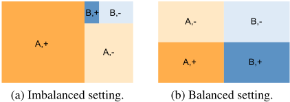
The balance between protected groups and labels is controlled by setting parameters pA, µA,+, µB,+. We visualize two such settings in Figure 2. For each dataset, we repeat the experiments 100 times, each with 10000 samples from a specific distribution setting.
It is also important to test the efficacy of our approach when experts have disparate performances or are extremely biased towards different groups. For binary classification with two protected groups, we create four "biased" classifiers/experts, where each is perfect (100% accurate) for one of the grouplabel subsets ({A, +}, {A, -}, {B, +}, {B, -}), and random (50% accurate) for the other three. Thus for each group-label subset, there is at least one perfect expert/classifier.
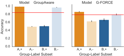
For imbalanced setting in Figure 2a, the results in Figure 3a shows that for GroupAware algorithm, the larger subsets {A, +} and {B, -} have nearly 100% accuracy while {A, -} and {B, +} have around 50% accuracy. The GroupAware algorithm, which runs only one MW instance per sensitive group, promotes selecting the perfect classifier for the larger group-label subset within each protected group. This leads to high error rates on the remaining subsets since their associated perfect classifiers are unlikely to be picked.
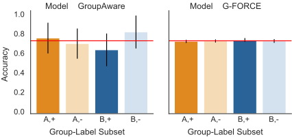
Even for a perfectly balanced setting (Figure 2b), GFORCE achieves a more balanced accuracy in each subset and a more stable behavior compared to GroupAware as in Figure 3b. Since the label distribution is balanced, {A,-} and {A, +} have the same accuracy when classifying an example from group A. GroupAware arbitrarily chooses between perfect classifier for {A,+} or {A,-} when classifying examples from group A, which leads to large deviations when considering errors on each more fine-grained subset (same analogy for group B). On the contrary, in both settings, G-FORCE is able to track the performance of the equalized odds on each group-label subset and compensate their differences in terms of accuracy. The side effect, as expected, is a slight decrease in accuracy. Due to the lack of space, we leave more experiment results in appendix. In appendix we also plot Pareto Curve to characterize the trade-off that can be achieved in G-FORCE.
| Adult | Compas | German | |||||||
|---|---|---|---|---|---|---|---|---|---|
| FPR | FNR | Regret | FPR | FNR | Regret | FPR | FNR | Regret | |
| GroupAware | 0.05± 0.01 | 0.17± 0.02 | 0.00± 0.00 | 0.20± 0.04 | 0.27± 0.04 | 0.01± 0.00 | 0.40± 0.13 | 0.21± 0.08 | 0.01± 0.01 |
| G-FORCE | 0.04± 0.01 | 0.08± 0.01 | 0.01± 0.00 | 0.18± 0.03 | 0.25± 0.04 | 0.01± 0.01 | 0.32± 0.15 | 0.18± 0.01 | 0.01± 0.01 |
(a) Imbalanced setting.
(b) Balanced setting.
Figure 3: The achieved accuracy on group-label subsets for imbalanced setting (pA = 0.9, µA,+ = 0.7, µB,+ = 0.3) and balanced Setting (pA = 0.5, µA,+ = 0.5, µB,+ = 0.5). Left: GroupAware. Right: G-FORCE. The vertical black line denotes the standard deviation. The red dashed line is the overall accuracy.
5.2 Case Study: Real Datasets
Datasets. We consider the Adult, German Credit and COMPAS datasets, all of which are commonly used by the fairness community. Adult consists of individuals' annual income measurements based on different factors. In the German dataset, people applying for credit from a bank are classified as "good" or "bad" credit based on their attributes. COMPAS provides a likelihood of recidivism based on a criminal defendant's history.
Creating Black-box Experts. The set of classifiers F that form the black-box experts are: Logistic Regression (LR), Linear SVM (L SVM), RBF SVM, Decision Tree (DT) and Multi-Layer Perceptron (MLP). These classifiers are trained using 70% of the data set. The remaining 30% of the dataset is set aside to simulate the online arrival of individuals. We compare our G-FORCE algorithm with the GroupAware in terms of regret and fairness. We repeated the experiments 1000 times for German and COMPAS, as well as 10 times for Adult, by randomizing the arrival sequence of individuals.
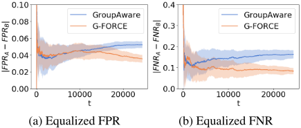
Results in Table-1 show a general improvement in fairness over the GroupAware algorithm, both in terms of equalized FPR and FNR, along with a small increase in regret. Although German and COMPAS have fewer examples, and thus the standard deviation is higher to make a conclusion, there is still a slight improvement over fairness with slight increase in regret. For Adult data set, we plot the performance of the algorithm over time (Figure 4). G-FORCE shows a clear improvement over GroupAware on both equalized FPR and equalized FNR over time with a slight increase in regret.
6 Discussion
In this paper, we introduce G-FORCE, a randomized MWbased algorithm achieving approximate equalized odds. Our algorithm gives a provable bound for the number of false positives and negatives obtained in an online stochastic setting, which could be potentially useful beyond the intended application of achieving fairness. We believe G-FORCE can be applied to a wide range of applications as it could work alongside with human decision makers and correct potential biases. A user could choose a λ to set a desirable trade-off between fairness and accuracy.
Future research could take on a more realistic case in which feedback is delayed for some number of rounds. For example, during the college admissions process, the performance of a student is generally evaluated at the end of each term, while colleges typically offer admission decisions in midyear. Similarly, when an individual applies for a loan, the bank often needs to wait for some time to know whether the applicant will default or not.
Acknowledgements
Dr. Cuesta-Infante is funded by the Spanish Government research fundings RTI2018-098743-B-I00 (MICINN/FEDER) and Y2018/EMT-5062 (Comunidad de Madrid)
@inproceedings{ijcai2021p416,
  title     = {Towards Reducing Biases in Combining Multiple Experts Online},
  author    = {Sun, Yi and Ramírez Díaz, Iván and Cuesta Infante, Alfredo and Veeramachaneni, Kalyan},
  booktitle = {Proceedings of the Thirtieth International Joint Conference on
               Artificial Intelligence, {IJCAI-21}},
  publisher = {International Joint Conferences on Artificial Intelligence Organization},
  editor    = {Zhi-Hua Zhou},
  pages     = {3024--3030},
  year      = {2021},
  month     = {8},
  note      = {Main Track},
  doi       = {10.24963/ijcai.2021/416},
  url       = {https://doi.org/10.24963/ijcai.2021/416},
}
TY - CPAPER TI - Towards Reducing Biases in Combining Multiple Experts Online AU - Sun, Yi AU - Ramírez Díaz, Iván AU - Cuesta Infante, Alfredo AU - Veeramachaneni, Kalyan T2 - Proceedings of the Thirtieth International Joint Conference on Artificial Intelligence, IJCAI-21 PB - International Joint Conferences on Artificial Intelligence Organization PY - 2021 SP - 3024 EP - 3030 DO - 10.24963/ijcai.2021/416 UR - https://doi.org/10.24963/ijcai.2021/416 ER -Copied
Machine-readable versions of this paper, for tools and AI agents:





