
Two-Sided Wasserstein Procrustes Analysis
Proceedings of the Thirtieth International Joint Conference on Artificial Intelligence. Main Track. Pages 3515-3521.
https://doi.org/10.24963/ijcai.2021/484
Keywords
- Machine Learning Applications: Bio/Medicine
- Machine Learning Applications: Applications of Unsupervised Learning
- Machine Learning: Transfer, Adaptation, Multi-task Learning
Abstract
Learning correspondence between sets of objects is a key component in many machine learning tasks.Recently, optimal Transport (OT) has been successfully applied to such correspondence problems and it is appealing as a fully unsupervised approach. However, OT requires pairwise instances be directly comparable in a common metric space. This limits its applicability when feature spaces are of different dimensions or not directly comparable. In addition, OT only focuses on pairwise correspondence without sensing global transformations. To address these challenges, we propose a new method to jointly learn the optimal coupling between twosets, and the optimal transformations (e.g. rotation, projection and scaling) of each set based on a two-sided Wassertein Procrustes analysis (TWP). Since the joint problem is a non-convex optimization problem, we present a reformulation that renders the problem component-wise convex. We then propose a novel algorithm to solve the problem harnessing a Gauss–Seidel method. We further present competitive results of TWP on various applicationscompared with state-of-the-art methods.
- [Alvarez-Melis and Jaakkola, 2018] David Alvarez-Melis and Tommi Jaakkola. Gromov-Wasserstein alignment of word embedding spaces. In Proceedings of the 2018 Conference on Empirical Methods in Natural Lan- guage Processing, pages 1881-1890, Brussels, Belgium, October-November 2018. Association for Computational Linguistics.
- [Alvarez-Melis et al., 2019] David Alvarez-Melis, Stefanie Jegelka, and Tommi S Jaakkola. Towards optimal trans- port with global invariances. In The 22nd International Conference on Artificial Intelligence and Statistics, pages 1870-1879. PMLR, 2019.
- [Arjovsky et al., 2017] Martin Arjovsky, Soumith Chintala, and Léon Bottou. Wasserstein gan. arXiv preprint arXiv:1701.07875, 2017.
- [Bruzzone and Marconcini, 2009] Lorenzo Bruzzone and Mattia Marconcini. Domain adaptation problems: A dasvm classification technique and a circular validation strategy. IEEE transactions on pattern analysis and ma- chine intelligence, 32(5):770-787, 2009.
- [Cavalli et al., 2007] Andrea Cavalli, Xavier Salvatella, Christopher M Dobson, and Michele Vendruscolo. Pro- tein structure determination from nmr chemical shifts. Proceedings of the National Academy of Sciences, 104(23):9615-9620, 2007.
- [Courty et al., 2017a] Nicolas Courty, Rémi Flamary, Amaury Habrard, and Alain Rakotomamonjy. Joint distribution optimal transportation for domain adaptation. In Advances in Neural Information Processing Systems, pages 3730-3739, 2017.
- [Courty et al., 2017b] Nicolas Courty, Rémi Flamary, Devis Tuia, and Alain Rakotomamonjy. Optimal transport for domain adaptation. IEEE transactions on pattern analysis and machine intelligence, 39(9):1853-1865, 2017.
- [Cuturi, 2013] Marco Cuturi. Sinkhorn distances: Light- speed computation of optimal transport. In Advances in neural information processing systems, pages 2292-2300, 2013.
- [Daumé III, 2009] Hal Daumé III. Frustratingly easy domain adaptation. arXiv preprint arXiv:0907.1815, 2009.
- [Fernando et al., 2013] Basura Fernando, Amaury Habrard, Marc Sebban, and Tinne Tuytelaars. Unsupervised visual domain adaptation using subspace alignment. In Proceed- ings of the IEEE international conference on computer vi- sion, pages 2960-2967, 2013.
- [Flamary et al., 2016] R Flamary, N Courty, D Tuia, and A Rakotomamonjy. Optimal transport for domain adap- tation. IEEE Trans. Pattern Anal. Mach. Intell, 2016.
- [Flamary et al., 2018] Rémi Flamary, Marco Cuturi, Nicolas Courty, and Alain Rakotomamonjy. Wasserstein discrim- inant analysis. Machine Learning, 107(12):1923-1945, 2018.
- [Gong et al., 2012] Boqing Gong, Yuan Shi, Fei Sha, and Kristen Grauman. Geodesic flow kernel for unsupervised domain adaptation. In 2012 IEEE Conference on Com- puter Vision and Pattern Recognition, pages 2066-2073. IEEE, 2012.
- [Grave et al., 2019] Edouard Grave, Armand Joulin, and Quentin Berthet. Unsupervised alignment of embeddings with wasserstein procrustes. In The 22nd International Conference on Artificial Intelligence and Statistics, pages 1880-1890, 2019.
- [Grippo and Sciandrone, 2000] Luigi Grippo and Marco Sciandrone. On the convergence of the block nonlinear gauss-seidel method under convex constraints. Operations research letters, 26(3):127-136, 2000.
- [Grippof and Sciandrone, 1999] Luigi Grippof and Marco Sciandrone. Globally convergent block-coordinate tech- niques for unconstrained optimization. Optimization meth- ods and software, 10(4):587-637, 1999.
- [Hoshen and Wolf, 2018] Yedid Hoshen and Lior Wolf. Non-adversarial unsupervised word translation. arXiv preprint arXiv:1801.06126, 2018.
- [Lample et al., 2018] Guillaume Lample, Alexis Conneau, Marc'Aurelio Ranzato, Ludovic Denoyer, and Hervé Jégou. Word translation without parallel data. In Inter- national Conference on Learning Representations, 2018.
- [Liu et al., 2013] Jia Liu, Cathy H. Xia, Ness B. Shroff, and Hanif D. Sherali. Distributed cross-layer optimization in wireless networks: A second-order approach. In 2013 Pro- ceedings IEEE INFOCOM, pages 2103-2111, 2013.
- [Liu et al., 2016] Jia Liu, Ness B. Shroff, Cathy H. Xia, and Hanif D. Sherali. Joint congestion control and routing opti- mization: An efficient second-order distributed approach. IEEE/ACM Transactions on Networking, 24(3):1404- 1420, 2016.
- [Mikolov et al., 2013] Tomas Mikolov, Quoc V. Le, and Ilya Sutskever. Exploiting similarities among languages for machine translation. CoRR, abs/1309.4168, 2013.
- [Overton and Womersley, 1992] Michael L Overton and Robert S Womersley. On the sum of the largest eigen- values of a symmetric matrix. SIAM Journal on Matrix Analysis and Applications, 13(1):41-45, 1992.
- [Pan et al., 2010] Sinno Jialin Pan, Ivor W Tsang, James T Kwok, and Qiang Yang. Domain adaptation via transfer component analysis. IEEE Transactions on Neural Net- works, 22(2):199-210, 2010. IJCAI
- [Schönemann, 1968] Peter H Schönemann. On two-sided or- thogonal procrustes problems. Psychometrika, 33(1):19- 33, 1968.
- [Sun et al., 2016] Baochen Sun, Jiashi Feng, and Kate Saenko. Return of frustratingly easy domain adaptation. In AAAI, volume 6, page 8, 2016.
- [Titouan et al., 2020] Vayer Titouan, Ievgen Redko, Rémi Flamary, and Nicolas Courty. Co-optimal transport. Ad- vances in Neural Information Processing Systems, 33, 2020.
- [Vandenberghe and Boyd, 1996] Lieven Vandenberghe and Stephen Boyd. Semidefinite programming. SIAM review, 38(1):49-95, 1996.
- [Wang and Mahadevan, 2008] Chang Wang and Sridhar Ma- hadevan. Manifold alignment using procrustes analysis. In Proc. of the 25th international conference on Machine learning, pages 1120-1127, 2008.
- [Zhang et al., 2017] Meng Zhang, Yang Liu, Huanbo Luan, and Maosong Sun. Earth mover's distance minimization for unsupervised bilingual lexicon induction. In Proc. of 2017 Conference on Empirical Methods in Natural Lan- guage Processing, pages 1934-1945, Copenhagen, Den- mark, 9 2017. Assoc. for Computational Linguistics.
References were extracted automatically from the PDF and may contain errors.
Full text extracted automatically from the PDF; figures, tables and equations may differ. The PDF is the version of record.
1 Introduction
Correspondence between sets of objects is useful in many machine learning problems, such as cross-lingual translation in natural language processing [Alvarez-Melis and Jaakkola, 2018; Grave et al., 2019] and protein alignment in computational biology [Wang and Mahadevan, 2008]. Recently, optimal transport (OT) has been successfully applied to solve such correspondence problems. It is appealing as a fully unsupervised approach, which not only derives correspondence between two sets geometrically, but also generates a wellfounded distance between two probability distributions. This distance, defined as the minimum transport cost between two point clouds endowed with different measures, serves naturally as a loss function in various applications, such as domain adaptation [Flamary et al., 2016; Courty et al., 2017a], and generative adversarial networks [Arjovsky et al., 2017; Lample et al., 2018].
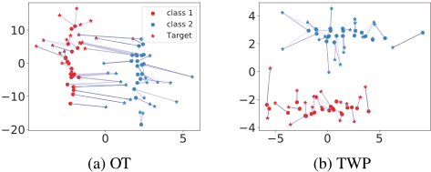
However, OT has limited applications as it requires pairwise instances directly comparable in a common metric space. If the feature dimensions of two instances are different, they cannot be compared; even if the dimensions are the same, direct comparison of instances may not be meaningful as they are typically from different spaces. This is not uncommon when instance representations are learned separately and independently from different training data. In addition, OT only focuses on pairwise coupling without sensing global transformations. Consider the example in Figure (1a), where there are two domains, source domain composed of filled circles and target domain composed of stars, each of which contains two classes distinguished with colors. Transformations (rotation, projection or scaling) must be done beforehand in order to find the optimal correspondence between source and target domains. Only after such transformations, can OT be applied effectively. Unfortunately, such transformations are typically unknown.
In this paper, we propose a novel method, Two-Sided Wasserstein Procrustes Analysis (TWP) to address above challenges. TWP is an integrated framework that jointly learn correspondences between two sets, and the optimal transformations of each set based on an extended form of Two-sided Procrustes Analysis. By exploiting advanced optimization methods, our method can eventually find the optimal correspondences between instances and obtain the latent transformations explicitly. With TWP, the correspondence between different dimensional datasets or from different spaces are enabled. Since the optimization problem related to TWP is non-convex, we present a novel reformulation that renders the problem component-wise convex. We show that TWP has elegant analytical solutions for each sub-problem, and the original problem can then be solved iteratively harnessing a Gauss-Seidel method. We experiment TWP over three applications: protein alignment, language alignment and domain adaptation and demonstrate competitive performance of TWP compared with state-of-the-art methods.
Related Work: [Mikolov et al., 2013] presents a supervised word embedding alignment method by learning a linear mapping between two sets using a well-aligned seed pairs and stochastic optimization. [Zhang et al., 2017] combines OT and Procrustes analysis for bilingual word embedding alignment, focusing on orthogonal transformation. They find that initializing the transformation matrix using Wasserstein GAN [Arjovsky et al., 2017] produces matching performance [Lample et al., 2018]. However, GAN has been criticized for difficulty on converging. [Hoshen and Wolf, 2018] presents a non-adversarial training using iterative matching methods. [Alvarez-Melis and Jaakkola, 2018] considers Gromov-Wasserstein distance for the unsupervised alignment problem. [Grave et al., 2019] proposes Wasserstein Procrustes by combining Wasserstein distance and Procrustes analysis to handle unsupervised alignment on different languages. Concurrent work proposed by [Alvarez-Melis et al., 2019] addresses the limitation of OT by involving global invariant transformations. To the best of our knowledge, TWP is the first attempt that integrate optimal transport with general forms of transformation including scaling, projection, and rotation and obtain simultaneously solutions for both correspondence learning and the latent transformation.
The rest of the paper is organized as follow. Section 2 presents main ideas of TWP. Section 3 covers analysis and algorithm to solve TWP. Section 4 demonstrates the performance of experiments. Sections 5 concludes the work.
2 Method
2.1 ProblemDescription
Consider two sets of samples, X = {xi}mi=1 and Y = {yj}nj=1 , separately drawn from different embedding spaces X ⊂ Rd1 and Y ⊂ Rd2 . The goal is to learn correspondences between sets X and Y . We are faced with two challenges: (1) samples in X and Y might not be directly comparable. This could be caused by many reasons, such as d1 ̸= d2 or distance between xi and yj is not meaningful; (2) no prior sample-wise correspondence information is available, leading to a fully unsupervised problem. In order to apply OT, we first need to find two transformation functions, Px ∈ Rd×d1 , and Py ∈ Rd×d2 that map X and Y respectively to a common latent d-dimensional space, where d is prespecified.
Our problem involves two levels of decisions that are mutually dependent. First, finding transformations Px and Py for embedding spaces X and Y such that d(Pxxi, Pyyj) is small for every paired samples (xi, yj ). Here, d(·, ·) is a general distance function and is defined by default as squared Euclidean distance, that is d(Pxxi, Pyyj) = ‖Pxxi -kPyyj‖2 , where k is a scalar variable; Second, given ̂X = PxX and ̂ Y = PyY , finding sample-wise correspondences between ̂X and ̂ Y via an assignment function A such that ̂ xA(i) → ̂ yj if ̂ xi and ̂ yj are in correspondence. We first discuss the solutions to each level of the problem, and then combine them together.
2.2 Two-sided Procrustes Analysis
Given two sets X and Y , when the correspondences between instances xi and yj are given, our transformation problem can be formulated as
If k = 1 and Px and Py are both permutation matrices (with d = d1 = d2), it is called Two-sided Procrustes Analysis first introduced by [Sch¨onemann, 1968]. Here we generalize the constraints on Px and Py that they do not have to be orthogonal square matrices. We also introduce a global scalar k to align the scaling of instances from two spaces. Note that it is a supervised approach since it needs the prior information of paired samples in X and Y .
2.3 Correspondence Between Samples
Given proper transformations that embed spaces X and Y into a common metric space, we can then harness OT for correspondence learning. We briefly introduce OT as follows.
Given two distributions µX and µY over spaces X and Y, and a transport cost function C : X ×Y → R+, OT is to find the optimal transport map Γ that pushes forward X onto Y so as to minimize a transport cost C(Γ). The minimum cost is known as Wasserstein or Earth Mover's Distance. Suppose µX and µY are only accessible through discrete samples, we then have the empirical distributions: µX = ∑ni=1 pxi δxi , µY = ∑mi=1 pyj δyj , where δxi is the Dirac function at location xi, and pxi (resp. pyj ) is probability mass associated to the i-th (resp. j-th) sample in set X (resp. Y). The OT problem can be formulated as
with Π := {Γ : Γ1n = µX, ΓT 1m = µY }. Here, Γ = [Γij] ∈ Rm×n specifies a probabilistic coupling or transport plan between xi and yj; C = [cij], whose term cij = C(xi, yj) denotes the cost of moving a probability mass from xi to yj; and 〈Γ,C〉F = ∑ij Γijcij is the Frobenius dot product between matrices Γ and C. Note that OT requires a common metric space where the distance between two instances from two sets xi and yj can be measured.
Recently, regularized approaches [Cuturi, 2013] have been shown to be efficient in solving Problem (2) via SinkhornKnoop algorithm with complexity O( n2 ϵ2 ). We hereby adopt a regularized discrete OT formulation by adding an entropic smoothing regularizer with hyperparameter ϵ, i.e. term -ϵH(Γ) to the objective function in (2), where
2.4 Two-sidedWasserstein Procrustes Analysis
To jointly learn transformations of each space as well as correspondence between instances, we formulate our TWP cost function as:
where β is the balance parameter, and Θ is a constraint to avoid trivial solutions for Px and Py to be specified later. We refer to J1 and J2 as costs associated respectively with 1) joint learning, scaling and matching; and 2) geometry preserving, which we next discuss in details.
Joint learning, Scaling andMatching, etc.
Given transformation Px and Py, J1 represents the optimal transport cost after transformation under the squared Euclidean distance:
where Dr and Dc denote the diagonal matrices and i-th diagonal value of Dr (Dc ) is defined as ∑nj=1 Γij (∑mj=1 ΓTij ).
Geometry Preserving
When learning the transformations, the local neighborhood relationship of either embedding space is not expected to be destroyed. In other words, the local geometry of either embedding space should be well preserved to avoid information loss. Inspired by [Flamary et al., 2018], we construct below the local adjacency relationship matrices W x and W y respectively for datasets X and Y .
where H(W) is the entropic smoothing regularizer for W defined in (3); ϵ2 and ϵ3 are the regularizer coefficients.
The geometry preserving function is formulated as:
where Lx = Dx - W x and Dx is a diagonal matrix in which the i-th row diagonal value is Dx ii = ∑j W x ij ; similarly, Ly = Dy -W y and Dy is a diagonal matrix in which the i-th row diagonal value is Dy ii = ∑j W y ij .
Combine Equations (5) and (8), we then have
where P := (Px Py), Z := (X 0 0 Y ) and LΓ is defined as
To avoid trivial solutions of Px, Py being zero matrices, we use the constraint:PxP T x +PyP T y = PP T = Id, where Id is the d × d identity matrix. Thus Θ := {P : PP T = Id}.
The joint optimization problem can then be written as:
3 Optimization
3.1 Semi-definite Programming
The inner problem of (11) is non-convex in the transformation matrix P . In this section, we present a convex relaxation which turns the inner problem into a semi-definite programming, and can help us find a solution to the non-convex problem.
It was shown in [Overton and Womersley, 1992] that the convex hull of Mp can be expressed as a convex set Me given by
where Me and Id -Me are both positive semi-definite. Each element inMp is an extreme point ofMe.
By changing the decision variables from P to Σ = P T P, we have the following relaxed form of Problem (11):
The advantage of the above relaxed formulation is twofold. First, under a fixed Γ and k, the inner problem of (13) is a semi-definite programming (SDP) on Σ, which can be solved in closed-form. Second, the objective function (13) is component-wise convex in Σ, k and Γ respectively, which gives us the theoretical advantages to solve the problem.
3.2 Learning Transformations
Under a fixed Γ and k, the inner problem of (13) is a semidefinite programming (SDP) on Σ:
The optima will be at one of those extreme points of the feasible region Me, precisely those matrices that have the form Σ = P T P where P ∈ Mp. As shown in [Vandenberghe and Boyd, 1996], the optimal solution has a closed form: Σ∗ = (P ∗ )T P ∗ where P ∗ is directly given by the matrix composed of eigenvectors corresponding to the d smallest eigenvalues of ZLΓ,kZ T . Since P = (Px Py), given P ∗ , the optimal transformations P ∗ x and P ∗ y to the original problem (11) follow immediately.
Note that the optimal P ∗ selects the eigenvectors for d smallest eigenvalues while abandoning the counterpart eigenvectors for (d1+d2-d) largest eigenvalues. It may leave the impression that it has abandoned a lot of information. However, P ∗ aims to find the transformations for X and Y so that the features of X and Y can be aligned as close as possible. Those divergent features in X and Y , leading to large eigenvalues in P ∗ , will be removed. Such phenomenon also occurs in domain adaptation [Daum´e III, 2009] where more identical words (which are also features) shared between source and target domain lead to higher prediction accuracy.
3.3 Learning Optimal Scaling
Under given P and Γ, the optimal scaling k∗ in Problem (13) can be derived via
where Ck is the pairwise squared Euclidean distance matrix between PxX and kPyY , i.e., Ck = ̂x1Tn + k2 1m̂y - 2k(PxX)T (PyY ), where ̂x = diag((PxX)T (PxX)),̂y = diag((PyY )T (PyY )), and diag(·) is a function which gives a column vector of the main diagonal elements of matrix. Thus Problem (15) becomes
which is a convex problem in k. Hence, the optimal k can be simply obtained via the first-order optimization condition:
In case of k being infinite, we restrict k ∈ [0, b], where b is a finite large number. The optimal scaling is then the solution to (15) projected onto range [0, b], i.e., max(0,min(k∗ , b)).
3.4 Learning Correspondences
Under given P and k, Problem (13) boils down to the following OT problem:
As discussed in Section 2.3, Γ∗ can be derived through OT using entropy regularizer (3).
3.5 Three-block Gauss-Seidel Method
Observe that the decision variables in Problem (13) are grouped into three blocks Γ, k and Σ. It is easily checked that the objective function J(Γ, k,Σ) is component-wise convex since the three subproblems (18), (16) and (14) are convex respectively in Γ, in k and in Σ. We can therefore solve the Problem (13) using a three-block Gauss-Seidel (GS) method, where the detailed procedure is given in Algorithm 1.
In words, the GS method [Grippof and Sciandrone, 1999], iteratively optimizes one block with the other blocks fixed (see lines 3-5 of Algorithm 1). A convergence proof for the GS method in the unconstrained case is given by [Grippof and Sciandrone, 1999] when the problem is jointly convex. In our case, Γ, k and Σ are constrained in convex regions and each subproblem is convex, but the Problem (13) is not jointly convex with respect to Γ, k and Σ. Fortunately, it was shown in [Grippo and Sciandrone, 2000] that, under the GS method, if it converges, every limit point must be a critical point under the condition that each subproblem is convex.
The initialization of Px, Py and k in Algorithm 1 is important. We use k0 = Tr(XT X) Tr(Y T Y ) as the initial value for k since it is the analytical solution to mink ‖X - kY ‖2F . The initialization strategy for Px and Py varies for different applications and datasets. For protein alignment and
Algorithm 1 TWP
Require:
- Data source: X ∈ Rd1×m,Y ∈ Rd2×n
- Dimension: d, Entropy regularization: ϵ
- Initialization of P: P 0
1: l = 0 2: loop 3: Γl = argminΓ J(Γ, kl , P l ) - ϵH(Γ) 4: P l+1 = argminP J(Γl , kl , P) 5: kl+1 = argmink J(Γl , k, P l ) 6: if converged then 7: break 8: end if 9: l = l +1 10: end loop 11: Return J(Γl , P l ), kl , P l , Γldomain adaptation experiments, Px and Py are suggested to be the first d largest components of projection matrices derived from PCA of X and Y [Fernando et al., 2013; Sun et al., 2016]. For cross-lingual translation, Px and Py are suggested to first use a small dataset to initialize as a warm start [Grave et al., 2019; Alvarez-Melis and Jaakkola, 2018; Alvarez-Melis et al., 2019]. Based on these suggestions, we use a simulated annealing strategy to initialize Px and Py.
4 Experiments
4.1 Protein Alignment
Protein 3D structure reconstruction is a key step of determining the Nuclear Magnetic Resonance (NMR) protein structure, which is a chain of amino acids. NMR techniques might determine multiple models since more than one configuration can be consistent with the distance matrix and the constraints. Therefore, the reconstructed result is a set of models rather than a single structure, and these structures are stored in the Protein Data Bank (PDB). Models derived from the same protein should be similar and comparisons between them indicate how well the protein conformation is determined by NMR. We refer to [Cavalli et al., 2007] for more details.
We use the data from [Wang and Mahadevan, 2008], where Glutaredoxin protein PDB-1G7O composed of 215 amino acids is used. The 3D sequences of two models 1G7O-1 (Protein 1) and 1G7O-10 (Protein 2) are illustrated in Figure (2a). The Protein 1 is much larger than the protein 2, and their orientation is very different. To apply TWP, we set the dimension of the common embedding space to be d = 3 (3D), d = 2 (2D) and d = 1 (1D), respectively. We apply TWP to align the models obtained from the same protein in the three settings. The 3D, 2D and 1D matching results of the two sequences are shown in Figure (2b),(2c),(2d), respectively. Observe that the two models match very well (in scales and orientations) after alignment by TWP using scaling, rotation and projection. This demonstrates the effectiveness of TWP in the protein alignment task.
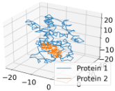
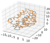
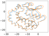
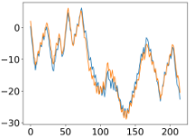
Figure 2: Protein Alignment with TWP.
4.2 Unsupervised Language Alignment
In this experiment, we evaluate TWP on the task of unsupervised language alignment. Given word embeddings pretrained from different monolingual corpora, the aim is to infer a bilingual dictionary in which each pair of words share similar semantic meanings. We use the same exact word vectors and evaluation datasets as [Alvarez-Melis and Jaakkola, 2018]. We focus on five language pairs as most related work reports: English to Spanish, French, German, Italian and Russian. We use a supervised Procrustes method as baseline where 5K pairs of words are known in prior. We compare TWP with previous state-of-the-art unsupervised methods for this task, namely, Adversarial training (ADV) method [Lample et al., 2018], Iterative Closest Point (ICP) method [Hoshen and Wolf, 2018], Gromov-Wasserstein (GW) [Alvarez-Melis and Jaakkola, 2018], Optimal Transport with Global Invariances (INVAROT) method [Alvarez-Melis et al., 2019] and Wasserstein Procrustes (WASSERSTEIN) approach [Grave et al., 2019]. All of the reported accuracy numbers are taken directly from their papers. CSLS denotes the cross-domain similarity local scaling method proposed by [Lample et al., 2018] to mitigate the hubness problem of nearest neighbors searching in high-dimensional spaces.
In this experiment, we set d = 230. We initialize the Px and Py via the simulated annealing as a warm start based on a small dataset of 5K most frequent words in each language. After obtaining the warm Px and Py, we then run TWP algorithm to get optimum. Table 1 demonstrates the performance of TWP is competitive to state-of-the-art methods.
4.3 Domain Adaptation
In this experiment, we evaluate TWP on two data adaptation datasets, namely Moons in [Bruzzone and Marconcini, 2009] and Office-Caltech in [Gong et al., 2012]. We set d = 2 in moons dataset and d = 120 in image dataset.
Moons
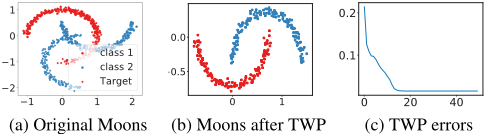
The Moons dataset is designed to perform a binary classification task and it is composed of two intertwined moons, each representing a class. The target dataset is constructed by rotating the source moons dataset with an angle ranging from 10 to 130 degrees, which generates 13 increasingly difficult adaptation tasks. The performance of Moons dataset is listed in Table (2), we could see that TWP always finds the optimal transformation (rotation) function and obtains accuracy of 100%. Figure (3a) depicts the original source and target domain datasets, Figure (3b) illustrates the transformed dataset, and Figure (3c) demonstrates the decreasing of TWP loss, i.e., Equation (11), along with the iterations until TWP algorithm converges. Observe that after TWP, the transformed source and target domain match well. This is not surprising because the target dataset is the rotation of source dataset and one strength of TWP to find such transformation. When there is prior knowledge that rotation of data exist in two domains, TWP can be the top choice. Similar results could be reached through the method in [Alvarez-Melis et al., 2019].
Noisy Moons
One column of noisy values, which follows Normal distribution N(0, 1), is added to the source moons dataset, while the target dataset remains unchanged. The source is of 3D while the target is of 2D, a setting which fails INVROT directly. We use Gromov-Wasserstein (G-W) [Alvarez-Melis and Jaakkola, 2018] and COOT [Titouan et al., 2020] as baseline methods. Observe that the accuracies obtained by G-W method and COOT both have a large variance by repeated runs while TWP is very stable, always obtaining perfect result. We report the average score in Table (3). G-W relies on the distance matrix between samples in two domains, and COOT requires the distance between source and target samples as well as the distance between source and target features. If features are noisy, which leads to the distance between samples and distance between features inaccurate, GW and COOT will have low performance. This experiment shows that TWP is a noise robust method by learning the optimal projections and correspondence of projected samples.
Office-Caltech
The Office-Caltech dataset is composed of images from 4 different domains: Amazon (A), Caltech (C), DSRL (D) and Webcam (W), each of which contains 10 classes with number of images ranging from 157 to 1123. Choosing one as source dataset and another one as target, we obtain 12 different source → target pairs. The features we use in the experiment are Surf features extracted from each image. We compare TWP with different methods listed as: Subspace Alignment (SA) [Fernando et al., 2013], Correlation Alignment (CA) [Sun et al., 2016], Transfer Component Analysis (TCA) [Pan et al., 2010], Optimal Transport with Domain Adaptation (OTDA) [Courty et al., 2017b], Joint Distribution Optimal Transport (JDOT) [Courty et al., 2017a]. We use 1-Nearest Neighbor (1NN) as the classifier since 1NN does not need tuning parameters. Table 4 demonstrates the performance of TWP on the Office-Caltech dataset. Observe that TWP outperforms other methods in 8 out of the 12 scenarios, showing the effectiveness of TWP in domain adaptation. Note that the performance of OTDA and TWP is comparable in most cases.
| EN-ES | EN-FR | EN-DE | EN-IT | EN-RU | |||||||
|---|---|---|---|---|---|---|---|---|---|---|---|
| Supervision | → | ← | → | ← | → | ← | → | ← | → | ← | |
| PROCRUSTES | 5K words | 77.6 | 77.2 | 74.9 | 75.9 | 68.4 | 67.7 | 73.9 | 73.8 | 47.2 | 58.2 |
| PROCRUSTES + CSLS | 5Kwords | 81.2 | 82.3 | 81.2 | 82.2 | 73.6 | 71.9 | 76.3 | 75.5 | 51.7 | 63.7 |
| ADV + CSLS | None | 75.7 | 79.7 | 77.8 | 71.2 | 70.1 | 66.4 | 72.4 | 71.2 | 37.1 | 48.1 |
| ADV + CSLS + REFINE | None | 81.7 | 83.3 | 82.3 | 82.1 | 74.0 | 72.2 | 77.4 | 76.1 | 44.0 | 59.1 |
| WASERSTEIN + CSLS | None | 82.8 | 84.1 | 82.6 | 72.9 | 75.4 | 73.3 | - | - | 43.7 | 59.1 |
| G-W | None | 81.7 | 80.4 | 81.3 | 78.9 | 71.9 | 72.8 | 78.9 | 75.2 | 45.1 | 43.7 |
| INVAROT + CSLS | None | 81.3 | 81.8 | 82.9 | 81.6 | 73.8 | 71.1 | 77.7 | 77.7 | 41.7 | 55.4 |
| ICP + CSLS | None | 81.1 | 82.1 | 81.5 | 81.3 | 73.7 | 72.7 | 77.0 | 76.6 | 44.4 | 55.6 |
| TWP + CSLS | None | 82.4 | 85.6 | 83.7 | 81.2 | 75.9 | 73.4 | 79.6 | 76.1 | 46.2 | 58.9 |
| Angle | SA | CA | TCA | OTDA | JDOT | TWP |
|---|---|---|---|---|---|---|
| 10 | 99.7 | 100 | 100 | 99.7 | 98.0 | 100 |
| 30 | 96.7 | 96.7 | 96.0 | 90.7 | 88.7 | 100 |
| 50 | 90.3 | 91.0 | 89.7 | 76.7 | 77.3 | 100 |
| 70 | 85.0 | 83.0 | 85.0 | 63.3 | 64.0 | 100 |
| 90 | 75.7 | 67.0 | 75.7 | 48.7 | 50.0 | 100 |
| 110 | 49.7 | 43.3 | 55.0 | 35.0 | 35.3 | 100 |
| 130 | 35.0 | 33.0 | 36.7 | 20.6 | 22.0 | 100 |
| AVG | 76.0 | 73.4 | 76.9 | 62.1 | 62.2 | 100 |
| G-W | COOT | TWP |
| 69.3 | 75.6 | 100 |
5 Conclusion
We propose TWP, an integrated method that jointly learn the optimal correspondence between two sets via OT, and the optimal transformations of each set via Two-sided Procrustes Analysis. We show that the joint learning problem is nonconvex but embraces a relaxed reformulation where the subproblems have nice convex properties. We develop a threeblock Gauss-Seidel method to solve the problem. We experiment TWP over three applications and demonstrate that TWP is effective and competitive to state-of-the-art work. It is possible to harness the convexity of subproblems and exploit higher order approaches, such as [Liu et al., 2013; Liu et al., 2016] for faster convergence, we will leave this as future investigation.
| Dataset | SA | CA | TCA | OTDA | JDOT | TWP |
|---|---|---|---|---|---|---|
| A→C | 40.2 | 25.4 | 40.0 | 40.2 | 39.9 | 41.2 |
| A→D | 39.3 | 26.8 | 31.8 | 40.1 | 37.6 | 41.4 |
| A→W | 39.9 | 26.8 | 41.7 | 37.3 | 38.0 | 40.3 |
| C→A | 41.3 | 23.6 | 39.8 | 52.7 | 48.1 | 53.0 |
| C→D | 45.4 | 26.1 | 44.6 | 47.8 | 49.7 | 47.1 |
| C→W | 36.6 | 23.7 | 36.9 | 46.4 | 43.4 | 46.4 |
| D→A | 35.4 | 28.8 | 32.9 | 32.4 | 32.8 | 35.7 |
| D→C | 32.3 | 30.0 | 31.5 | 32.0 | 31.7 | 33.9 |
| D→W | 88.5 | 84.4 | 84.7 | 88.8 | 82.7 | 80.7 |
| W→A | 32.6 | 26.2 | 29.4 | 33.7 | 37.6 | 37.7 |
| W→C | 29.0 | 22.6 | 29.2 | 34.1 | 33.1 | 34.6 |
| W→D | 89.5 | 84.1 | 91.7 | 92.4 | 89.8 | 79.0 |
| AVG | 45.8 | 35.7 | 44.5 | 48.2 | 47.0 | 47.6 |
@inproceedings{ijcai2021p484,
  title     = {Two-Sided Wasserstein Procrustes Analysis},
  author    = {Jin, Kun and Liu, Chaoyue and Xia, Cathy},
  booktitle = {Proceedings of the Thirtieth International Joint Conference on
               Artificial Intelligence, {IJCAI-21}},
  publisher = {International Joint Conferences on Artificial Intelligence Organization},
  editor    = {Zhi-Hua Zhou},
  pages     = {3515--3521},
  year      = {2021},
  month     = {8},
  note      = {Main Track},
  doi       = {10.24963/ijcai.2021/484},
  url       = {https://doi.org/10.24963/ijcai.2021/484},
}
TY - CPAPER TI - Two-Sided Wasserstein Procrustes Analysis AU - Jin, Kun AU - Liu, Chaoyue AU - Xia, Cathy T2 - Proceedings of the Thirtieth International Joint Conference on Artificial Intelligence, IJCAI-21 PB - International Joint Conferences on Artificial Intelligence Organization PY - 2021 SP - 3515 EP - 3521 DO - 10.24963/ijcai.2021/484 UR - https://doi.org/10.24963/ijcai.2021/484 ER -Copied
Machine-readable versions of this paper, for tools and AI agents:





