
Multi-series Time-aware Sequence Partitioning for Disease Progression Modeling
Proceedings of the Thirtieth International Joint Conference on Artificial Intelligence. Main Track. Pages 3581-3587.
https://doi.org/10.24963/ijcai.2021/493
Keywords
- Machine Learning: Explainable/Interpretable Machine Learning
- Machine Learning Applications: Applications of Unsupervised Learning
- Machine Learning: Time-series; Data Streams
Abstract
Electronic healthcare records (EHRs) are comprehensive longitudinal collections of patient data that play a critical role in modeling the disease progression to facilitate clinical decision-making. Based on EHRs, in this work, we focus on sepsis -- a broad syndrome that can develop from nearly all types of infections (e.g., influenza, pneumonia). The symptoms of sepsis, such as elevated heart rate, fever, and shortness of breath, are vague and common to other illnesses, making the modeling of its progression extremely challenging. Motivated by the recent success of a novel subsequence clustering approach: Toeplitz Inverse Covariance-based Clustering (TICC), we model the sepsis progression as a subsequence partitioning problem and propose a Multi-series Time-aware TICC (MT-TICC), which incorporates multi-series nature and irregular time intervals of EHRs. The effectiveness of MT-TICC is first validated via a case study using a real-world hand gesture dataset with ground-truth labels. Then we further apply it for sepsis progression modeling using EHRs. The results suggest that MT-TICC can significantly outperform competitive baseline models, including the TICC. More importantly, it unveils interpretable patterns, which sheds some light on better understanding the sepsis progression.
- [Baytas et al., 2017] Inci M Baytas, Cao Xiao, Xi Zhang, Fei Wang, Anil K Jain, and Jiayu Zhou. Paient subtyping via time-aware lstm networks. In SIGKDD. ACM, 2017.
- [Berkhin, 2005] Pavel Berkhin. A survey on pagerank com- puting. Internet mathematics, 2(1):73-120, 2005.
- [Boyd et al., 2011] Stephen Boyd, Neal Parikh, and Eric Chu. Distributed optimization and statistical learning via the alternating direction method of multipliers. Now Pub- lishers Inc, 2011.
- [Che et al., 2015] Zhengping Che, David Kale, Wenzhe Li, Mohammad Taha Bahadori, and Yan Liu. Deep computa- tional phenotyping. In SIGKDD. ACM, 2015.
- [Choi et al., 2016a] Edward Choi, Mohammad Taha Ba- hadori, Andy Schuetz, Walter F Stewart, and Jimeng Sun. Doctor ai: Predicting clinical events via recurrent neural networks. In MLHC, pages 301-318, 2016.
- [Choi et al., 2016b] Edward Choi, Mohammad Taha Ba- hadori, Jimeng Sun, et al. Retain: An interpretable pre- dictive model for healthcare using reverse time attention mechanism. In NIPS, pages 3504-3512, 2016.
- [Cuturi, 2011] Marco Cuturi. Fast global alignment kernels. In Proceedings of the 28th international conference on ma- chine learning (ICML-11), pages 929-936, 2011.
- [Fleuren et al., 2020] Lucas M Fleuren, Thomas LT Klausch, et al. Machine learning for the prediction of sep- sis: a systematic review and meta-analysis of diagnostic test accuracy. Intensive care medicine, pages 1-18, 2020.
- [Friedman et al., 2001] Jerome Friedman, Trevor Hastie, and Robert Tibshirani. The elements of statistical learning, volume 1. Springer series in statistics New York, 2001.
- [Friedman et al., 2008] Jerome Friedman, Trevor Hastie, and Robert Tibshirani. Sparse inverse covariance estima- tion with the graphical lasso. Biostatistics, 2008.
- [Giuliano, 2007] Karen K Giuliano. Physiological monitor- ing for critically ill patients: testing a predictive model for the early detection of sepsis. American Journal of Critical Care, 16(2):122-130, 2007.
- [Hallac et al., 2017] David Hallac, Sagar Vare, Stephen Boyd, and Jure Leskovec. Toeplitz inverse covariance- based clustering of multivariate time series data. In SIGKDD, pages 215-223, 2017.
- [Ho et al., 2014] Joyce Ho, Cheng Lee, and Joydeep Ghosh. Septic shock prediction for patients with missing data. Management Information Systems, 5(1), 2014.
- [Kumar et al., 2006] Anand Kumar, Daniel Roberts, et al. Duration of hypotension before initiation of effective an- timicrobial therapy is the critical determinant of survival in human septic shock. Critical care medicine, 2006.
- [Li et al., 2012] Yuan Li, Jessica Lin, and Tim Oates. Visu- alizing variable-length time series motifs. In Proceedings of the 2012 SIAM, pages 895-906. SIAM, 2012.
- [Li et al., 2018] Jia Li, Yu Rong, Helen Meng, et al. Tatc: Predicting alzheimer's disease with actigraphy data. In Proceedings of the 24th ACM SIGKDD, 2018.
- [Lin et al., 2019] Chen Lin, Julie S. Ivy, and Min Chi. Multi- layer facial representation learning for early prediction of septic shock. In IEEE BigData, 2019.
- [Lipton et al., 2015] Zachary C Lipton, David C Kale, and Randall Wetzel. Learning to diagnose with lstm recurrent neural networks. arXiv preprint arXiv:1511.03677, 2015.
- [Lipton et al., 2016] Zachary Lipton, David Kale, and Ran- dall Wetzel. Directly modeling missing data in sequences with RNNs: Improved classification of clinical time series. JMLR, 2016.
- [Lobov et al., 2018] Sergey Lobov, Nadia Krilova, et al. La- tent factors limiting the performance of semg-interfaces. Sensors, page 1122, 2018.
- [Lobov et al., 2019] Sergey Lobov, Nadia Krilova, et al. EMG data for gestures Data Set, 2019. https://archive. ics.uci.edu/ml/datasets/EMG+data+for+gestures#. Link
- [Meinshausen and Bühlmann, 2006] Nicolai Meinshausen and Peter Bühlmann. High-dimensional graphs and variable selection with the lasso. Ann. Statist., 2006.
- [Nadeau and Bengio, 2003] Claude Nadeau and Yoshua Bengio. Inference for the generalization error. Machine learning, 52(3):239-281, 2003.
- [Reynolds, 2009] Douglas A Reynolds. Gaussian mixture models. Encyclopedia of biometrics, 741, 2009.
- [Severson et al., 2020] Kristen A Severson, Lana M Chahine, et al. Personalized input-output hidden markov models for disease progression modeling. In Machine Learning for Healthcare Conference, 2020.
- [Singer et al., 2016] Mervyn Singer, Clifford S Deutschman, et al. The third international consensus definitions for sep- sis and septic shock (sepsis-3). Jama, 315, 2016.
- [Smyth, 1997] Padhraic Smyth. Clustering sequences with hidden markov models. In Advances in neural information processing systems, pages 648-654, 1997.
- [Sohn et al., 2020] Hyunwoo Sohn, Kyungjin Park, and Min Chi. Mulan: Multilevel language-based representation learning for disease progression modeling. In IEEE In- ternational Conference on Big Data, 2020.
- [Tintinalli et al., 1985] Judith E Tintinalli, Gabor D Kelen, J Stephan Stapczynski, et al. Emergency medicine: a com- prehensive study guide. Mcgraw-hill New York, 1985.
- [Viterbi, 1967] Andrew Viterbi. Error bounds for convolu- tional codes and an asymptotically optimum decoding al- gorithm. IEEE transactions on Information Theory, 1967.
- [Yang et al., 2017] Jinxing Yang, Jianhong Pan, and Jun Li. semg-based continuous hand gesture recognition using gmm-hmm and threshold model. In IEEE ROBIO, 2017.
- [Zhang et al., 2019] Yuan Zhang, Yang Xi, Ivy Julie, and Min Chi. Attain: Attention-based time-aware lstm net- works for disease progression modeling. In IJCAI, 2019. IJCAI
References were extracted automatically from the PDF and may contain errors.
Full text extracted automatically from the PDF; figures, tables and equations may differ. The PDF is the version of record.
1 Introduction
Electronic health records (EHRs) are comprehensive longitudinal collections of patients' health data. The extensive application of EHRs in medical systems has accelerated the development of various computational methods for understanding patients' medical history, identifying interesting cohorts, predicting potential risks, evaluating interventions, etc. [Che et al.2015, Choi et al.2016b, Zhang et al.2019] Among them, disease progression modeling (DPM) is a crucial task, which monitors disease development, predicts future risks based on historical events, and assists clinicians in making effective interventions. Given its importance, many recent works aim to develop automated solutions for DPM using machine learning techniques [Choi et al.2016a,Choi et al.2016b,Baytas et al.2017,Lin et al.2019]. In this work, we focus on modeling the progression of an extremely challenging disease - sepsis, a life-threatening organ dysfunction and a leading cause of death worldwide [Singer et al.2016]. Without timely diagnosis and proper intervention, sepsis can progress from infection to septic shock, which is the most severe stage with a mortality rate as high as 50% [Sohn et al.2020]. Contrarily, 80% of the sepsis deaths can be prevented with timely diagnosis and interventions [Kumar et al.2006].
Despite great importance, modeling the sepsis progression with EHRs is particularly challenging. Specifically, whether a patient has sepsis is not directly observable, and its symptoms are often hidden by medical "expert blind spots" [Tintinalli et al.1985]. Moreover, different patient groups may show diverse symptoms. For example, although one common sign of sepsis is fever, for the young, old, or immune system weakened patients, their body temperature may be low or normal when sepsis is present. Thus, our key research question is: Can the modeling of sepsis progression be automated? So far, the DPM of sepsis is generally modeled by supervised learning [Fleuren et al.2020], which relies on a large amount of fine-grained moment-by-moment labeled data. Such labeled data are not only time and expertise intensive, but also often infeasible to be acquired [Giuliano2007, Singer et al.2016].
In this work, we utilize an unsupervised learning approach to automatically model the sepsis progression, which is formulated as a subsequence partitioning problem to partition and cluster the subsequences in EHRs simultaneously. More importantly, we expect the discovered subsequence clusters to be interpretable because in healthcare domains, it is usually more essential to learn discriminative and interpretable patterns that reflect the disease progression than to merely induce a prediction model. Recently, Severson et al. employed a hidden Markov model (HMM)-based method to learn the Parkinson's progression, which encoded prior knowledge to learn the latent states and then used post-hoc analysis to interpret the states [Severson et al.2020]. In this work, we learn the inerpretable DPM by leveraging a novel subsequence clustering method, Toeplitz inverse covariance-based clustering (TICC) [Hallac et al.2017]. TICC employs inverse covariance matrices and constrains these matrices to be block-wise Toeplitz to model the time-invariant structural patterns in each cluster. It outperforms both distance-based methods, e.g., dynamic time warping (DTW) [Cuturi2011] or rule-based motif discovery [Li et al.2012]), and model-based methods, e.g., Gaussian mixture models (GMM) [Reynolds2009] or hidden Markov models [Smyth1997]. Moreover, TICC has successfully discovered interpretable patterns in various applications, such as driving patterns in traffic data [Hallac et al.2017] and physical activity patterns in Alzheimer's data [Li et al.2018].
Despite the great success of TICC, there are two major challenges when applying it to EHRs: 1) TICC takes a single time series as input, whereas most EHRs consist of multiple series as a collection of visits from different patients. Applying TICC to each visit independently may lead to inconsistent patterns across different visits, while concatenating all visits to be a single series may introduce some undesired patterns at the joints between adjacent visits. Therefore, in this work, we extend the TICC by considering multi-series inputs and refer to it as Multi-series TICC (M-TICC); 2) The records in EHRs are generally collected with irregular time intervals, varying from seconds to days. For example, the interval between two consecutive records in our EHRs ranges from 0.94 seconds to 28.19 hours. Hence, it is essential to consider irregular time intervals for capturing latent progressive patterns of a targeted disease [Baytas et al.2017]. However, the TICC ignores the intervals and encourages the consecutive records to be assigned into the same cluster. Consequently, we further extend M-TICC by incorporating time-awareness for the consistency between consecutive records, which is denoted as Multi-series, Time-aware TICC (MT-TICC).
The effectiveness of MT-TICC is first validated with a case study involving a real-world hand gesture dataset (sEMG). Like EHRs, sEMG is human-oriented with multi-series and irregular time intervals; more importantly, it has moment-bymoment ground-truth labels for each record, which can be employed to validate the MT-TICC derived clusters. Our results show that MT-TICC significantly outperforms the stateof-the-art models, including the TICC. Then we applied MTTICC for sepsis progression modeling using the real-world EHRs. To evaluate the MT-TICC derived clusters, we incorporate them into the original EHRs for a task of septic shock early prediction. The results show significantly improved prediction performance comparing to using original EHRs or using the clusters learned by TICC. Furthermore, the clusters derived by MT-TICC convey meaningful insights and shed some light on better understanding the sepsis progression.
2 Methodology
2.1 Preliminaries
Given a dataset with N multivariate sequences, denoting the n-th sequence (length T n ) as {xn1 , . . . , xnT n}, where xnt ∈ Rm is the t-th event, we aim to simultaneously partition and cluster the events based on their latent patterns. Without loss of generality, supposing there are K clusters in the dataset, we will learn a mapping from each event xnt to a certain cluster k ∈ {1, . . . ,K}. Since the events in a sequence are consecutive and each event is dependent on its neighbors, instead of mapping each event independently, we investigate events in a sliding window ω ≪ T n . For xnt , its preceding events within ω, i.e., Xnt = {xnt-ω+1 , . . . , xnt }, are extracted for determining which cluster k the event xnt belongs to.
To learn the clustering mapping in an unsupervised manner, we treat each Xnt as a mω-dimension random variable (obtained by concatenating the ω events in Xnt ) and optimally fit all variables into K Gaussian distributions, with the k-th fitted distribution corresponding to the k-th cluster. Of note, each Xnt will only contribute (belong) to one distribution (cluster). The TICC [Hallac et al.2017] characterizes each distribution by determining its mean and inverse covariance matrix. Specifically, for all K distributions, determining the optimal mean vectors {µk|k = 1, . . . ,K} is equivalent to matching each event to an optimal cluster, which leads to the clustering assignment results P = {Pk|k = 1, . . . ,K}, where Pk ⊂ {1, . . . , T n } denotes the indices of (sliding window) events belonging to the cluster k; meanwhile, determining the optimal {Θk|k = 1, . . . ,K} is to estimate K inverse covariancematriceswith block-wise Toeplitz constraints. It is worth noting that the inverse covariance matrix is used rather than the covariance matrix because it models conditional dependencies and can easily introduce a graph structure during the matrix learning [Hallac et al.2017], which can substantially decrease the number of parameters to reduce the risk of overfitting [Meinshausen and B¨uhlmann2006]. Each Θk for a cluster k is constrained to be block-wise Toeplitz, which composes of ω sub-blocks A(i) ∈ Rm×m, i ∈ [0, ω - 1]:
The sub-block A(i) represents the partial correlations among m features between timestamps t and t + i. For example, the (p, q)-th entry in A(i) indicates the partial correlation between the p-th feature at t and the q-th feature at t + i, where p, q ∈ {1, . . . ,m}. The block-wise Toeplitz constraints enable Θk to capture time-invariant structural patterns within Xnt .
2.2 M-TICC
The original TICC learns time-invariant structural patterns to simultaneously partition and cluster over a single sequence. To apply it to multi-series input, we can either treat each sequence independently or concatenate them as one sequence. However, both strategies are not optimal. When treating each sequence independently, the learned patterns across different sequences can be inconsistent due to sequence discrepancies, while concatenating all sequences will introduce undesired patterns due to the artificial joints between neighboring sequences. To handle this issue, we adapt the TICC for jointly partitioning and clustering across difference sequences to explicitly learn the shared patterns, which is denoted as Multiseries TICC (M-TICC), as formulated in Eq.(1). Note that when N = 1, Eq.(1) will degenerate into the original TICC.
The roles of three terms in Eq.(1) are detailed as follows: · Log-likelihood term measures the probability that Xnt be-
- longs to cluster k. Since Xnt ∼ N(µk,Θ-1 k ), we have:
- Consistency term detailed in Eq.(3) encourages neighbored events {Xt-1,Xt} to be assigned into the same cluster.
Herein, 1{t - 1 /∈ Pk} is an indicator function, which is 1 if Xnt-1 does not belong to the same cluster as Xnt , otherwise it is 0. By minimizing Eq.(3), neighbored events belonging to different clusters will be penalized. β is a weight parameter.
- Sparsity term controls the sparseness of Θk via a l1-norm, which selects the most significant variables to represent the time-invariant structural patterns that can effectively prevent overfitting. λ is a sparsity regularization coefficient.
2.3 MT-TICC
Both M-TICC and TICC assume neighboring events having equal time intervals. However, the intervals between neighbored events can vary greatly, ranging from seconds to days in EHRs. Specifically, two events with a shorter interval would more likely belong to the same cluster comparing to those with longer intervals. Thus, it is essential to consider the time interval irregularity in the consistency term. To address this problem, we incorporate Time-awareness into the consistency term to make it interval-dependant, which is denoted as MTTICC. The modified objective function is presented in Eq.(4).
- Time-aware consistency term encourages the consecutive events {Xt-1,Xt} with shorter time interval to be assigned into the same cluster, which is defined as:
Herein, we introduce a decay function, i.e., 1/log(e+∆T n t ), which can adaptively relax the penalization of the consistency constraint as the interval ∆T n t between neighboring events becomes larger [Baytas et al.2017]. The nonlinear monotonically decreasing manner of the decay function enables us to control the impact of intervals over the consistency term.
2.4 Optimization
To solve the objective functions shown in Eq.(1) and Eq.(4), we adopt the expectation-maximization (EM) framework to iteratively learn the cluster assignments P and the structural patterns Θ until convergence. Specifically, in E-step, Θ is fixed to learn P, then Eq.(1) and Eq.(4) degenerate into a form with only the log-likelihood term and the consistency term. It can be solved by dynamic programming to find a minimum cost Viterbi path [Viterbi1967] for all sequences. The computational complexity is O(KT), which is closely linear since the K is generally small. In M-step, P is fixed to learn the Θ, then Eq.(1) and Eq.(4) degenerate into a form with only the log-likelihood term and the sparsity term, which can be considered as a typical graphical lasso problem [Friedman et al.2008] with a Toeplitz constraint over Θ. It can be solved by an alternating direction method of multipliers (ADMM) [Boyd et al.2011]. During implementation, we found that ADMM can derive the solution with a moderate time cost. Given our entire EHRs (4,224,567 events with 14 features), it converges in ∼20 iterations with each iteration costing ∼120s (Intel i7-8700k with 32GB memory).
3 Experiments
3.1 ACase Study
Data Description and Preprocessing
The hand gesture dataset we employed in this case study contains multichannel surface electromyographic (sEMG) signals collected from 36 participants, each of whom performed a series of hand gestures twice [Lobov et al.2019]. For every timestamp in a series of sEMG signals, the corresponding gesture is taken as the ground-truth label. We carried out three steps to preprocess the data: 1) Smoothing signals: the raw sEMG signals were recorded per millisecond with high volatility. To obtain more stable data, a common approach is to smooth the signals via a sliding window. Referring to the settings in [Lobov et al.2018], we applied a 100 ms window with the step size of 50 ms. Inside the sliding window, the signals were smoothed by the root-mean-squared values. 2) Slicing and shuffling gestures: five labeled gestures were sliced for analysis, including hand at rest (rest), wrist flexion (left), wrist extension (right), radial deviation (up), and ulnar deviation (down). To ensure the data covers more complex scenarios similar to EHRs, we randomly shuffled the gestures order. Note that the order of timestamps within each gesture and its interval to the previous gesture remain unchanged. 3) Selecting features: the five targeted gestures were mainly monitored by four muscles located in the forearm [Lobov et al.2018]. Therefore, we selected the corresponding four data channels as features and normalized them to the range of [0, 1]. Finally, our data consists of 72 sequences with 14,441 timestamps. The intervals range from [50, 5450] ms.
Validating the Effectiveness of MT-TICC
Based on the sEMG data, we evaluated the effectiveness of MT-TICC. Specifically, for the training data, we learned cluster assignment for each timestamp and compared it against the ground-truth label; for the test data, based on the learned clustering model, we followed Eq.(2) to calculate the probability belonging to each cluster and then assigned the data to the cluster with the maximal probability.
- Baselines: We compared our MT-TICC to 1) M-TICC which takes multi-series as input without time-awareness and 2) six other baselines including: TICC which randomly concatenates all sequences as a single input, I-TICC which treats each sequence independently, TICC(β=0) which is a competitive baseline reflected in [Hallac et al.2017] without the consistency term, model-based Gaussian mixture model (GMM) [Reynolds2009] and a hidden Markov model using GMM for emissions (GMM-HMM) [Yang et al.2017], and a distancebased dynamic time warping (DTW) [Cuturi2011].
| Method | Training Data | Test Data | ||||||||||||||
|---|---|---|---|---|---|---|---|---|---|---|---|---|---|---|---|---|
| Acc | Rec | Prec | F1 | NMI | ARI | Hom | Com | Acc | Rec | Prec | F1 | NMI | ARI | Hom | Com | |
| DTW | .208 | .211 | .229 | .186 | .002 | .000 | .002 | .002 | .212 | .213 | .322 | .232 | .016 | .000 | .004 | .017 |
| GMM | .556 | .609 | .584 | .573 | .387 | .296 | .369 | .408 | .563 | .621 | .674 | .628 | .430 | .316 | .399 | .468 |
| GMM-HMM | .610 | .610 | .637 | .616 | .422 | .318 | .415 | .429 | .614 | .642 | .660 | .635 | .447 | .373 | .444 | .450 |
| TICC(β = 0) | .686 | .708 | .686 | .677 | .453 | .405 | .446 | .461 | .674 | .694 | .674 | .664 | .444 | .393 | .436 | .451 |
| I-TICC | .845 | .912 | .878 | .879 | .810 | .750 | .781 | .845 | .554 | .554 | .558 | .517 | .399 | .318 | .374 | .430 |
| TICC | .696 | .721 | .696 | .687 | .475 | .423 | .467 | .484 | .677 | .698 | .677 | .668 | .451 | .398 | .444 | .459 |
| M-TICC | .710 | .735 | .710⋆ | .702 | .491 | .442† | .484† | .499⋆ | .685 | .709 | .685† | .677 | .458 | .408 | .450 | .465 |
| MT-TICC | .728⋆ | .747⋆ | .728⋆ | .721⋆ | .512⋆ | .473⋆ | .505⋆ | .519⋆ | .699† | .721⋆ | .699⋆ | .690⋆ | .474⋆ | .430⋆ | .466⋆ | .481⋆ |
.
| Method | Training Data | Test Data | ||||||||||||||
|---|---|---|---|---|---|---|---|---|---|---|---|---|---|---|---|---|
| Acc | Rec | Prec | F1 | NMI | ARI | Hom | Com | Acc | Rec | Prec | F1 | NMI | ARI | Hom | Com | |
| TICC | .549 | .618 | .549 | .527 | .297 | .224 | .281 | .315 | .519 | .621 | .519 | .499 | .288 | .213 | .273 | .304 |
| M-TICC | .570 | .634 | .570⋆ | .552 | .318 | .246† | .303† | .335⋆ | .533 | .648 | .533⋆ | .516 | .316 | .195 | .292 | .316 |
| MT-TICC | .602⋆ | .647⋆ | .602⋆ | .584⋆ | .344⋆ | .294⋆ | .332⋆ | .357⋆ | .571⋆ | .656⋆ | .571⋆ | .557⋆ | .338⋆ | .242⋆ | .321⋆ | .357⋆ |
Table 1: Clustering results in sEMG with: (a) overall data and (b) data over joints connecting two subsequences. The best results in test data are in bold. ⋆ denotes p-value < 0.01 and † denotes p-value < 0.05 when comparing M-TICC and MT-TICC against TICC, respectively.
- Parameters: All the model parameters were determined by Bayesian information criteria (BIC) [Friedman et al.2001]. In MT-TICC, the cluster number K was 11; the window size ω was 2; the sparsity and consistency coefficients λ and β were 1e-5 and 4, respectively. For a fair comparison, the optimal parameters in other methods were determined by BIC as well. · Metrics: The results were evaluated via 1) classification metrics: accuracy (Acc), recall (Rec), precision (Prec), and F1-score (F1), which treated the clustering as a multi-class classification to compare the results against the ground-truth labels. Specifically, the metrics were weighted by the respective size of each label; and 2) clustering metrics: normalized mutual information (NMI), adjusted random index (ARI), homogeneity score (Hom), and completeness score (Com). We repeated the 5-fold cross-validation ten times and conducted a corrected paired t-test [Nadeau and Bengio2003] to compare MT-TICC and M-TICC against the TICC.
- Results: We compared MT-TICC against other methods first across the whole trajectories and then specifically around the joints connecting two subsequences with different groundtruth labels. Since the events in a sequence are consecutive and dependent on neighboring events, the switch of patterns around the joints is more challenging to be identified. To do so, we defined a tolerance window (tol) around the joints and evaluated the results within the tol. In this study, tol is set as 5, with 39.4% of the overall data counted as joints.
Table 1(a) reports the results of different methods for overall data. Among the six baselines, I-TICC performs the best in training data while the second-worst in test data. It might because the individual sequence cannot provide adequate information to cover all variation across different sequences. Taking together both training and test data, TICC performed the best among the baselines. When comparing M-TICC and MT-TICC against TICC: ⋆ denotes p-value < 0.01 and † denotes p-value < 0.05. The results demonstrated that both MTTICC and M-TICC outperformed the TICC by taking multiseries as input. Furthermore, equipped with time-awareness, MT-TICC performed the best among all methods. Specifically, compared to TICC, MT-TICC improved by ∼ 3% and ∼ 2% in training and test data, respectively. Table 1(b) shows the results for data over joints within the tol. Herein, we merely compared the best baseline, i.e., TICC, due to the page limit. As expected, clustering over joints is much harder compared to overall data. The improvement of MT-TICC versus TICC was ∼ 6% in training data and ∼ 5% in test data. The results suggested that the time-awareness of MT-TICC could effectively capture the switch of subsequence clusters, which is especially important in modeling the disease progression.
3.2 Experiments with EHRs
Our EHRs were collected by Christiana Care Health System (CCHS) from Jul. 2013 to Dec. 2015, with each sequence being a patient's visit consisting of a series of events. To evaluate the results derived fromMT-TICC, we treated the learned clusters as additional features for a task of septic shock early prediction. If the learned clusters sufficiently capture the sepsis progression, we expect that combining them with the original EHRs would improve the prediction performance.
Data Preprocessing
In our EHRs, 52,919 visits (4,224,567 events) with suspected infection was identified as sepsis-related study cohort. Note that the rules employed for identifying the suspected infection and tagging septic shock were provided by two leading clinicians with extensive sepsis experience from CCHS and Mayo Clinic. The selected cohort was preprocessed as follows:
- Selecting features: 14 features related to the sepsis progression were selected as suggested by clinicians: 1) Vital signs: systolic blood pressure (SBP), mean arterial pressure (MAP), respiratory rate (RR), oxygen saturation (PulOx), heart rate (HR), temperature (Temp); 2) Lab results: white blood cell (WBC), bilirubin (Bili), blood urea nitrogen (BUN), lactate (Lac), creatinine (Creat), platelet (Plat), neutrophils (Bands); and 3) Intervention: fraction of inspired Oxygen (FiO2).
- Handling the missing data: The events in each visit were collected with irregular intervals, ranging from 0.94 seconds to 28.19 hours. Specifically, different features are measured with varying frequencies, which causes some features to be unavailable and missing from certain events. On average, the missing rate of our data is ∼80.37%. Herein, we handled the absence of data by carrying forward, i.e., filling the missing entries as the last observation until the next observed value, with the remaining missing entries filled as the mean value.
- Tagging the septic shock visits: Identifying the septic shock visits is a challenging task. Though the diagnosis codes, e.g., ICD-9, are widely used for clinical labeling, solely relying on the codes can be problematic: they have proven to be limited in reliability since the coding practice is mainly used for administrative and billing purpose [Ho et al.2014]. Based on the Third International Consensus Definitions for Sepsis and Septic Shock [Singer et al.2016], our domain experts identified septic shock when either of the following two conditions was met: 1) Persistent hypertension through two consecutive readings (≤ 30 minutes apart), including SBP < 90 mmHg, MAP < 65mmHg, and decrease in SBP ≥ 40 mmHg within an 8-hour period; or 2) Any vasopressor administration.
By combing ICD-9 codes and domain experts' rules, we identified 1,869 shock and 23,901 non-shock visits. Considering the highly imbalanced ratio, we conducted a stratified random sampling on non-shock visits while keeping the same underlying distribution of age, sex, ethnicity, and stay duration. Finally, the dataset was narrowed down to 3,738 visits (1,869 shock and 1,869 non-shock) with 145,421 events.
Experimental Settings
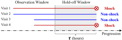
Herein, our goal is to predict septic shock as early as possible, which is defined as: given the observation of a patient's visit until τ hours before an endpoint, we will predict whether or not the visit will develop into septic shock τ hours later. For septic shock visits, the endpoint is the onset time of septic shock while for non-shock visits, the endpoint is the end of sequences. As shown in Figure 1, the τ hours leading up to the endpoint is denoted as hold-off window.
We employed long short-term memory (LSTM) as the prediction model since extensive previous works have demonstrated its preferable performance in EHRs modeling [Lipton et al.2015,Baytas et al.2017, Sohn et al.2020]. Different inputs to the LSTMwere compared, including: 14 Original features (O) vs. original features with additional Cluster-based features (O+C) learned from three TICC-based methods, i.e., TICC, M-TICC, and MT-TICC. In MT-TICC, the cluster number K was determined as 6 via BIC; therefore, six additional features were generated for each event, which measure the probabilities of the event belonging to each cluster based on Eq.(2). For test data, the additional features were generated based on the clustering models learned from training data. BIC determined the K for M-TICC and TICC as 7 and 9, respectively. The other parameters involved in the three TICCbased methods were tuned based on BIC as well: for example, in MT-TICC, the window size ω was 3; the sparsity and consistency coefficients λ and β were 1e-8 and 10, respectively. We implemented LSTM with Keras and tuned the parameters by grid search. All models were evaluated by repeating the
3-fold cross-validation ten times. The results were compared over τ ∈ [12, 24) and τ ∈ [24, 36] to validate whether septic shock can be predicted at least 12 hours or a day in advance. The metrics of Acc, Rec, Prec, F1, and AUC were employed.
Results and Interpretations
- Septic shock early prediction: The early prediction results are shown in Table 2, which suggested the effectiveness of (O+C) features: (O+C) learned with the three TICC-based methods all outperformed the (O)-only. Especially, for the recall, MT-TICC improved by ∼ 8% and ∼ 7% comparing to (O) when τ ∈ [12, 24) and τ ∈ [24, 36], respectively. When comparing M-TICC and MT-TICC to TICC: ⋆ denotes the p-value < 0.01 and † indicates the p-value < 0.05. The results showed that the multi-series input can effectively learn the shared patterns across different sequences since M-TICC outperformed the TICC, and the time-awareness is effective in modeling the irregular intervals since MT-TICC performed better than M-TICC. Equipped with both multi-series and time-awareness, MT-TICC achieved the best performance.
We further visualized the F1 score and AUC when varying τ from 1 hour to 36 hours before the septic shock onset, as shown in Figure 2. As τ increases, it becomes harder for early prediction across all models. The figures showed the advantage of (O+C) learned by three TICC-based methods comparing to Original (O)-only. Especially, it is demonstrated that the MT-TICC performed the best. When τ is larger, the gaps between MT-TICC and other methods are more apparent.
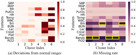
- Interpretation for MT-TICC derived patterns: For each cluster learned by MT-TICC, we calculated the mean value of each feature: if the value is abnormal, we measured its deviation from the normal range. As shown in Figure 3(a): the darker the color, the more abnormal the feature is. We ranked the 6 clusters from the least severe (Cluster 1) to the most severe (Cluster 6) based on the deviations. Referring to the criteria suggested by our domain experts, we obtained interpretations for each cluster as shown in Table 3. The clusters reflected the complications that could happen simultaneously.
The missing rates for the features in each cluster are visualized in Figure 3(b): the darker the color, the higher the missing rate. Then we analyzed how the missing rates are related to the patterns learned by MT-TICC. Since the structural patterns Θ can be represented as graphs, we calculated the PageRanks [Berkhin2005] to measure the importance of features in each cluster. The features with the maximum PageRanks are highlighted with yellow boxes in Figure 3(b). An interesting finding is that the features with the maximum PageRanks usually have the highest missing rates, which indicates the MT-TICC has similar effects with missing indicators [Lipton et al.2016] to capture structural patterns.
We further analyzed the transitions between the clusters.
| Hold-off Window τ ∈ [12, 24) | Hold-off Window τ ∈ [24, 36] | ||||||||||
|---|---|---|---|---|---|---|---|---|---|---|---|
| Features | Acc | Rec | Prec | F1 | AUC | Acc | Rec | Prec | F1 | AUC | |
| (O) | Original | .743(.016) | .728(.022) | .753(.022) | .739(.015) | .813(.015) | .704(.012) | .701(.020) | .709(.017) | .703(.013) | .778(.018) |
| TICC | .757(.012) | .748(.016) | .765(.021) | .755(.010) | .825(.014) | .713(.013) | .717(.025) | .715(.015) | .714(.015) | .783(.018) | |
| (O+C) | M-TICC | .772(.011)⋆ | .767(.020)† | .778(.011) | .771(.013)⋆ | .837(.010) | .730(.014)⋆ | .735(.022)† | .732(.016)† | .731(.015)⋆ | .797(.017)⋆ |
| MT-TICC | .790(.010)⋆ | .806(.025)† | .784(.015) | .793(.011)⋆ | .852(.012)† | .761(.010)⋆ | .773(.023)† | .758(.023)† | .763(.007)⋆ | .825(.011)⋆ | |
| Cluster Idx | Interpretations |
|---|---|
| 1 | Metabolic Dysfunction |
| 2 | Renal Dysfunction |
| 3 | Non-temperature Physiological Response Infection, Cellular Response, Renal Dysfunction |
| 4 | Non-temperature Physiological Response Infection, Metabolic Dysfunction |
| 5 | Non-temperature Physiological Response Infection, Metabolic Dysfunction, Renal Dysfunction, Gastrointestinal Dysfunction |
| 6 | Non-temperature Physiological Response Infection, Cellular Response Infection, Metabolic Dysfunction, Renal Dysfunction |
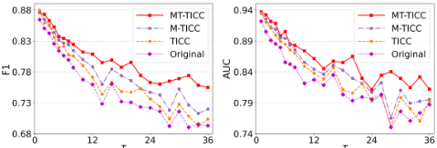
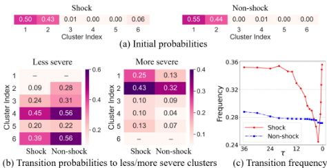
Figure 4(a) indicates that the initial probabilities of shock and non-shock visits are quite similar. Figure 4(b) displays the probabilities transiting to Less severe or More severe clusters. For example, in Cluster 2: for a shock visit, the probability of transiting to less severity (Cluster 1) is 0.09, while for the non-shock visit, the probability is 0.28; meanwhile, for a shock visit, the probability of transiting to more severity (Cluster 3, Cluster 4, Cluster 5, and Cluster 6) is 0.43, while for the non-shock visit, the probability is 0.32. In general, non-shock visits have higher probabilities transiting to less severity and lower probabilities transiting to more severity comparing to shock counterparts. Figure 4(c) shows the transition frequencies when sepsis progress, with τ decreasing from 36 hours to 0.2 hours. The non-shock visits are stable when τ varies. In contrast, the shock visits have high frequencies at the beginning; when τ decreases, the visits more likely turn into the severe cluster and hardly get out, thus the transition frequencies decrease; the frequencies surge in 2 hours before the onset of septic shock, which possibly arises from augmented clinical interventions. As a result, MT-TICC can effectively cluster subsequences and capture the differences in cluster transitions between shock and non-shock visits.
4 Conclusions
In this paper, we improved the TICC by incorporating multiseries input (M-TICC) and time-awareness (MT-TICC). The effectiveness of MT-TICC was validated first in hand gesture clustering and then in septic shock early prediction using EHRs. Experimental results showed that the multi-series input and time-awareness in MT-TICC contributed to better learning of the clustering patterns. In addition, with the time-awareness, MT-TICC performed superior to M-TICC and also significantly outperformed the original TICC. Moreover, the clusters derived by MT-TICC conveyed interpretable insights that could help clinicians better understand the sepsis progression. We will further explore varying-length sliding windows and introduce attentions to our model in future.
Acknowledgements
This research was supported by the NSF Grants: #1522107, #1651909, #1660878, #1726550 and #2013502.
@inproceedings{ijcai2021p493,
  title     = {Multi-series Time-aware Sequence Partitioning for Disease Progression Modeling},
  author    = {Yang, Xi and Zhang, Yuan and Chi, Min},
  booktitle = {Proceedings of the Thirtieth International Joint Conference on
               Artificial Intelligence, {IJCAI-21}},
  publisher = {International Joint Conferences on Artificial Intelligence Organization},
  editor    = {Zhi-Hua Zhou},
  pages     = {3581--3587},
  year      = {2021},
  month     = {8},
  note      = {Main Track},
  doi       = {10.24963/ijcai.2021/493},
  url       = {https://doi.org/10.24963/ijcai.2021/493},
}
TY - CPAPER TI - Multi-series Time-aware Sequence Partitioning for Disease Progression Modeling AU - Yang, Xi AU - Zhang, Yuan AU - Chi, Min T2 - Proceedings of the Thirtieth International Joint Conference on Artificial Intelligence, IJCAI-21 PB - International Joint Conferences on Artificial Intelligence Organization PY - 2021 SP - 3581 EP - 3587 DO - 10.24963/ijcai.2021/493 UR - https://doi.org/10.24963/ijcai.2021/493 ER -Copied
Machine-readable versions of this paper, for tools and AI agents:





