
SpanConv: A New Convolution via Spanning Kernel Space for Lightweight Pansharpening
Proceedings of the Thirty-First International Joint Conference on Artificial Intelligence. Main Track. Pages 841-847.
https://doi.org/10.24963/ijcai.2022/118
Keywords
- Computer Vision: Machine Learning for Vision
- Machine Learning: Convolutional Networks
- Computer Vision: Computational photography
- Machine Learning: Applications
Abstract
Standard convolution operations can effectively perform feature extraction and representation but result in high computational cost, largely due to the generation of the original convolution kernel corresponding to the channel dimension of the feature map, which will cause unnecessary redundancy. In this paper, we focus on kernel generation and present an interpretable span strategy, named SpanConv, for the effective construction of kernel space. Specifically, we first learn two navigated kernels with single channel as bases, then extend the two kernels by learnable coefficients, and finally span the two sets of kernels by their linear combination to construct the so-called SpanKernel. The proposed SpanConv is realized by replacing plain convolution kernel by SpanKernel. To verify the effectiveness of SpanConv, we design a simple network with SpanConv. Experiments demonstrate the proposed network significantly reduces parameters comparing with benchmark networks for remote sensing pansharpening, while achieving competitive performance and excellent generalization. Code is available at https://github.com/zhi-xuan-chen/IJCAI-2022 SpanConv.
- [Aiazzi et al., 2002] Bruno Aiazzi, Luciano Alparone, Ste- fano Baronti, and Andrea Garzelli. Context-driven fu- sion of high spatial and spectral resolution images based on oversampled multiresolution analysis. IEEE Trans- actions on geoscience and remote sensing, 40(10):2300- 2312, 2002.
- [Alparone et al., 2004] Luciano Alparone, Stefano Baronti, Andrea Garzelli, and Filippo Nencini. A global qual- ity measurement of pan-sharpened multispectral imagery. IEEE Geoscience and Remote Sensing Letters, 1(4):313- 317, 2004.
- [Alparone et al., 2008] Luciano Alparone, Bruno Aiazzi, Stefano Baronti, Andrea Garzelli, Filippo Nencini, and Massimo Selva. Multispectral and panchromatic data fu- sion assessment without reference. Photogrammetric En- gineering & Remote Sensing, 74(2):193-200, 2008.
- [Boardman, 1993] Joseph Boardman. Automating spectral unmixing of aviris data using convex geometry concepts. In Summaries of the 4th Annual JPL Airborne Geoscience Workshop, volume 1, pages 11-14, 1993.
- [Deng et al., 2021] Liang-Jian Deng, Gemine Vivone, Cheng Jin, and Jocelyn Chanussot. Detail injection-based deep convolutional neural networks for pansharpening. IEEE Transactions on Geoscience and Remote Sensing, 59(8):6995-7010, 2021.
- [Garzelli and Nencini, 2009] Andrea Garzelli and Fil- ippo Nencini. Hypercomplex quality assessment of multi/hyperspectral images. IEEE Geoscience and Remote Sensing Letters, 6(4):662-665, 2009.
- [Ghazali et al., 2011] Rozaida Ghazali, Abir Jaafar Hussain, and Panos Liatsis. Dynamic ridge polynomial neural net- work: Forecasting the univariate non-stationary and sta- tionary trading signals. Expert Systems with Applications, 38(4):3765-3776, 2011.
- [Haase and Amthor, 2020] Daniel Haase and Manuel Amthor. Rethinking depthwise separable convolutions: How intra-kernel correlations lead to improved Mo- bileNets. In The IEEE/CVF Conference on Computer Vision and Pattern Recognition (CVPR), June 2020.
- [He et al., 2019] Lin He, Yizhou Rao, Jun Li, Jocelyn Chanussot, Antonio Plaza, Jiawei Zhu, and Bo Li. Pan- sharpening via detail injection based convolutional neu- ral networks. IEEE Journal of Selected Topics in Applied Earth Observations and Remote Sensing, 12(4):1188- 1204, 2019.
- [Howard et al., 2017] Andrew G. Howard, Menglong Zhu, Bo Chen, Dmitry Kalenichenko, Weijun Wang, Tobias Weyand, Marco Andreetto, and Hartwig Adam. Mo- bilenets: Efficient convolutional neural networks for mo- bile vision applications. arXiv preprint arXiv:1704.04861, 2017.
- [Jin et al., 2022] Cheng Jin, Liang-Jian Deng, Ting-Zhu Huang, and Gemine Vivone. Laplacian pyramid networks: A new approach for multispectral pansharpening. Infor- mation Fusion, 78:158-170, 2022.
- [Krizhevsky et al., 2012] Alex Krizhevsky, Ilya Sutskever, and Geoffrey E Hinton. Imagenet classification with deep convolutional neural networks. Advances in neural infor- mation processing systems, 25:1097-1105, 2012.
- [Lolli et al., 2017] Simone Lolli, Luciano Alparone, An- drea Garzelli, and Gemine Vivone. Haze correction for contrast-based multispectral pansharpening. IEEE Geo- science and Remote Sensing Letters, 14(12):2255-2259, 2017.
- [Masi et al., 2016] Giuseppe Masi, Davide Cozzolino, Luisa Verdoliva, and Giuseppe Scarpa. Pansharpening by convo- lutional neural networks. Remote Sensing, 8(7):594, 2016.
- [Meyer, 2000] C. D. Meyer. Matrix Analysis and Applied Linear Algebra Book and Solutions Manual. Matrix Anal- ysis and Applied Linear Algebra Book and Solutions Man- ual, 2000.
- [T.-J. Zhang and Vivone, 2022] T.-Z. Huang J. Chanussot T.- J. Zhang, L.-J. Deng and G. Vivone. A triple-double con- volutional neural network for panchromatic sharpening. IEEE Transactions on Neural Networks and Learning Sys- tems, 2022.
- [Vivone et al., 2018] Gemine Vivone, Rocco Restaino, and Jocelyn Chanussot. Full scale regression-based injection coefficients for panchromatic sharpening. IEEE Transac- tions on Image Processing, 27(7):3418-3431, 2018.
- [Vivone et al., 2020] Gemine Vivone, Mauro Dalla Mura, Andrea Garzelli, Rocco Restaino, Giuseppe Scarpa, Mag- nus Orn Ulfarsson, Luciano Alparone, and Jocelyn Chanussot. A new benchmark based on recent advances in multispectral pansharpening: Revisiting pansharpening with classical and emerging pansharpening methods. IEEE Geoscience and Remote Sensing Magazine, 2020.
- [Vivone, 2019] Gemine Vivone. Robust band-dependent spatial-detail approaches for panchromatic sharpening. IEEE transactions on Geoscience and Remote Sensing, 57(9):6421-6433, 2019.
- [Wald, 2002] Lucien Wald. Data fusion: definitions and ar- chitectures: fusion of images of different spatial resolu- tions. Presses des MINES, 2002.
- [Wei et al., 2017] Yancong Wei, Qiangqiang Yuan, Xi- angchao Meng, Huanfeng Shen, Liangpei Zhang, and Michael Ng. Multi-scale-and-depth convolutional neural network for remote sensed imagery pan-sharpening. In 2017 IEEE International Geoscience and Remote Sensing Symposium (IGARSS), pages 3413-3416. IEEE, 2017.
- [Yang et al., 2017] Junfeng Yang, Xueyang Fu, Yuwen Hu, Yue Huang, Xinghao Ding, and John Paisley. Pannet: A deep network architecture for pan-sharpening. In Proceed- ings of the IEEE/CVF International Conference on Com- puter Vision, pages 5449-5457, 2017.
- [Zhang et al., 2019] Yongjun Zhang, Chi Liu, Mingwei Sun, and Yangjun Ou. Pan-sharpening using an efficient bidi- rectional pyramid network. IEEE Transactions on Geo- science and Remote Sensing, 57(8):5549-5563, 2019.
References were extracted automatically from the PDF and may contain errors.
Full text extracted automatically from the PDF; figures, tables and equations may differ. The PDF is the version of record.
1 Introduction
High-spatial-resolution (HR) multispectral (MS) images are the database that reflects changes in geographic information. However, satellite sensors cannot provide HR-MS images due to payload and bandwidth constraints. Pansharpening, a task of fusing HR panchromatic (PAN) images with simultaneously captured low-spatial-resolution (LR) MS images to ob-
ing mineral exploration, agricultural surveying, geological monitoring, etc. Existing pansharpening approaches can be divided into two categories: hand-crafted feature-based methods and deep learning-based methods.
LR-MS and PAN images are frequently represented by features backed with conventional image processing knowledge in hand-crafted feature-based approaches [Lolli et al., 2017;
∗Contact Author
Vivone, 2019; Vivone et al., 2018]. However, these features have limited representational power due to their simple struc-
ear fitting ability of convolutional neural networks (CNNs), deep learning feature-based approaches [Masi et al., 2016; Yang et al., 2017; He et al., 2019; Deng et al., 2021; Jin et al., 2022; T.-J. Zhang and Vivone, 2022] can automatically extract features from training data and express the complex nonlinearity of data. A comprehensive review can be found in [Vivone et al., 2020].
To improve the performance of CNNs, deeper architectures with millions of parameters are proposed while increasing the computational burden. To balance the computational cost and performance of CNNs, several works, such as group convolution [Krizhevsky et al., 2012], deeply separable convolution [Howard et al., 2017] and blueprint separable convolutions (BSConv) [Haase and Amthor, 2020] attempt to form a more advanced convolution module by modifying the representation of convolution kernels. In addition, complex and deep CNNs will have overfitting problem that cannot be ignored, which leads to poor performance of the model in the face of unknown data, limiting its application in real scenarios.
In this paper, we propose a SpanConv module based on SpanKernel, whose generation process is analogous to the spanning process in linear algebra. In detail, we learn the navigated kernels as the basis vectors, then span the kernel space by corresponding coefficients to create a kernel slice along each input channel dimension. We observed that standardconvolution-generalized kernels distribution could depict as a subspace in the kernel space, which inspired us to cut down the number of navigated kernels, thus reducing the computational parameters with trade-offs of accuracy. The contributions of this work are two-fold:
- We construct a kernel space that approximates the standard convolution kernel space through spanning, and remove the possible redundancy of the standard convolution kernel, which significantly reduces the number of parameters. To the best of our knowledge, the proposed SpanConv method has the fewest network parameters (only about 16,000 parameters) while maintaining competitive pansharpening performance.
- We further analyze the proposed SpanConv from the perspective of subspace in linear algebra, and point out the
optimal number of navigated kernels by empirical experiments. Also, the better generalization of the given approach is verified comparing with recent state-of-theart (SOTA) pansharpening techniques.
2 RelatedWorks andMotivation
The standard convolution kernel needs to realize the joint mapping of channel correlation and spatial correlation. Its parameters involve spatial and channel dimensions, which are inefficient and prone to redundancy. In AlexNet [Krizhevsky et al., 2012], where group convolution is proposed, the standard convolution procedure is divided into g sets of smaller sub-operations that can be executed in parallel, thus reducing the computation complexity. In MobileNets [Howard et al., 2017], authors build a simplified architecture through the depth-wise separable convolution (DSC) module. The DSC module decomposes the standard convolution into depthwise convolution and pointwise convolution, thus significantly reducing the parameters. In blueprint separable convolutions (BSConv) [Haase and Amthor, 2020], it is found that many convolution kernels exhibit the same structure after visualizing the learned convolution kernels. Therefore, BSConv uses only a template called a "blueprint" convolution kernel to generate the convolution kernel (denoted as BlueKernel from hereon) and achieves magnificent parameters cut down.
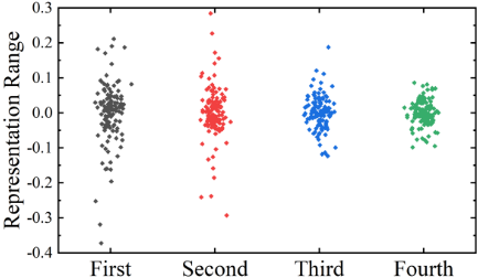
Motivation. As the number of convolutional channels increases, learnable parameters dramatically intensify. This problem is unavoidable for deep convolutional neural networks and imposes a tremendous computational load on devices. Naturally, not all parameters are indispensable, which can be observed in the specific pansharpening task. In Fig. 2, we use the standard convolution to replace the SpanConv in our proposed network and reshape the trained kernels into a matrix Fi (please refer to the definition introduced in Sect. 3.3). Then we apply the principal component analysis (PCA) to the Fi, and draw the scatter distribution of the first four principal components of each kernel, demonstrating the low rank of Fi. The results show that the first two components manifest strong representation ability, of which the remaining components are weak. This observation further verifies the correlation of standard kernels along the channel dimension. Considering this, we attempt to generate a kernel space that can approximate the standard convolution kernel by the linear combination of basis vectors, thereby alleviating the problem of computational parameters.
3 Methodology
In what follows, we will first give several Definitions and one Lemma, then further propose our SpanKernel base on them.
3.1 Background and Definitions
The Preparation of Linear Algebra. To illustrate the given method, we need to first present some basic concepts in linear algebra, which can be found from the book in [Meyer, 2000]
Definition 1. If β = {v1, v2, · · · , vr} is r linearly independent vectors in Rk2 , then we have the space spanning:
By Definition 1, we then define the Definition 2,
Definition 2. If vi ∈ Rk2 , λi ∈ R, and r ≤ k2 where r, k2 ∈ N, then the following space
is a subspace of Rk2 .
Lemma 1. In Definition 2, if r = k2 , the space Lr could completely represent Rk2 , when r < k2 , the space Lr could not completely represent Rk2 .
By Definition 1, Definition 2 and Lemma 1, we use them into the analysis for the kernel space, and we get the following Definition 3 and three important conclusions.
Definition 3. For easy analysis, we may reshape the Fi ∈ RCin×k×k to Cin kernel vector kj ∈ Rk2 , correspondingly define the following kernel space:
which are distributed in Rk2 .
According to Definition 2 and Lemma 1, we define vi = ¯Ki, if β = { ¯K1, ¯K2, · · · , ¯Kr} is r linearly independent vectors in Rk2 kernel space:
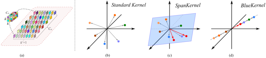
Standard Kernel. For standard kernel, the parameters in one layer is Cout × Cin × k2 , where the Cout is represents the number of output channel. Any of kernel vector in standard kernel space can be represented by linearly independent vectors in β when r = k2 , as the Fig. 1 (b) shows.
BlueKernel. In order to reduce parameters, the BlueKernel [Haase and Amthor, 2020] takes an extreme approach. It only learns a ¯K1 ∈Rk2 as basis vector. Then, using the Cin learnt coefficients, the authors expand the basis vector to Cin convolution kernels. In mathematics, its essence is equal to the linear subspace spanned by β when r = 1, as illustrated in Fig. 1 (d). Considering the parameters for the coefficients, the parameters of BlueKernel in a layer are Cout×(Cin×1+k2×1), which are tiny. And as far as we know, the paper of BSConv did not describe its method in terms of math theory.
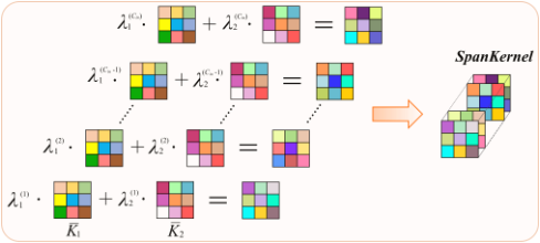
SpanKernel. For the proposed SpanKernel, we have known only two linearly independent vectors (β when r = 2) can greatly represent the standard kernel space according to the PCA analysis in Sec. 2, as Figure. 1 (c) shows. Its specific generation method is displayed in Fig. 3. The parameters of SpanKernel in a layer are Cout × (Cin × 2 + k2 × 2). And it can be concluded from Fig. 1 (c) and (d), the representation ability of SpanKernel is better than BlueKernel prominently.
3.2 Generation of SpanKernel
By the above analysis, we intend to only learn two independent kernels as the bases 1 , then extend the two basis kernels ¯Ki, i = 1, 2 to Cin channels by learnable coefficients and finally span the two sets of navigated kernels by their linear combination to construct the so-called SpanKernel, aiming to represent all standard kernels approximately with tolerable errors. For the detailed procedure, please refer to Fig. 3.
1 The case of more independent kernels will be discussed in the experiments.
3.3 Analysis
The Selection of the Number of Navigated Kernels. Here, we discuss the number of navigated kernels in different situations. We reshape and view the kernel Fi ∈ RCin×k×k to Fi ∈ RCin×k2 in each input feature channel as a set of vectors, as illustrated in Fig. 1 (a), where i indicates the output channel index. Usually, Fi is a non-full-rank matrix, thus satisfying Rank(Fi) ≤ k2 (generally, Cin > k2 ).
When Rank(Fi) = k2 , as mentioned in Sec. 3.1, we could employ r = k2 independent vectors to completely represent any vector of Fi. Thus, the number of navigated kernel vectors, i.e., N, is also equal to Rank(Fi) = k2 . In this situation, the number of parameters with SpanConv is Cout × (Cin × k2 + k2 × k2 ), which is greater than that with standard convolution, Cout × Cin × k2 .
When Rank(Fi) < k2 , the N still needs to be equal to Rank(Fi) for representing standard kernel space.
In summary, the N is always equal to Rank(Fi), and the number of parameters will reduce when the N decreases. To balance the representation ability discussed in the Sec. 2 and the parameters, we finally set N = 2 in our experiments.
Comparison with Benchmark Convolution Kernels. With the above background, we analyze the modeling process of SpanKernel and compare it with standard kernel and prior module BlueKernel [Haase and Amthor, 2020] as follows.
For standard convolutions, the kernel in an output channel is arbitrarily scattered in Rk2 space. In the training process, the algorithm directly learns a set of fixed kernel vectors by back-propagation, as Fig. 1 (b) shows. It is self-evident from knowledge of linear algebra that a collection of linearly independent bases is capable of describing any vector in its corresponding space. In the proposed method, we view the kernel vectors that exist in the subspace of the Rk2 space, and use a pair of navigated vectors to span this subspace, as Fig. 1 (c) illustrates. If the kernel generation has single navigated BlueKernel Cout(k2 +Cin)
| Kernel Type | Parameters |
| Standard Kernel SpanKernel | CoutCink2 Cout(2k2 +2Cin) |
Table 1: The parameters of the three types of kernels.
kernel, our SpanKernel degenerates into BlueKernel, as Fig. 1 (d) shows. This operation can further reduce the parameters, however, its representation capability is limited. The parameters of the three kernels are displayed in Tab. 1.
3.4 Proposed LightNet
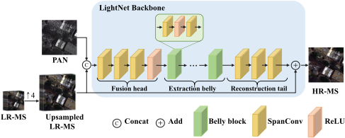
In this section, we introduce the proposed LightNet, in which all convolutions are implemented by SpanConv that are realized by replacing the standard kernel with SpanKernel. As shown in Fig. 4, our model has three components, i.e., a fusion head, an extraction belly and a reconstruction tail.
The fusion head consists of three convolution layers with an increasing channel number. It inputs concatenated PAN and upsampled LR-MS images and outputs a preliminary fusion feature. The Cout ×Cin of three layers are 9×9, 20×9 and 32 × 20, respectively. To introduce fractional linearity, a ReLU layer is set at the end of the fusion head.
The extraction belly receives features from the visual backbone and performs detail extraction. It is composed by several belly blocks. Each block is made up of two convolution layers with a sandwiched ReLU layer. The Cout × Cin of the convolution layer in belly are all 32 × 32, and the block number defaults to 2.
The part of reconstruction tail comprises three convolution layers with decreasing channel number. It produces compensated features, which are added to the upsampled LR-MS image for the final fusion outcome. In particular, the Cout×Cin of the three layers are 16×32, 8×16 and 8×8, respectively.
Network Training. Our overall objective is to train LightNet to perform the fusion of LR-MS and PAN images, and obtain a high quality HR-MS image. We exploit the ℓ1 distance between the network prediction and the ground truth (GT) image to supervise the reconstruction process. Besides, the Adam optimizer is utilized with a learning rate that decays by 0.75 every 120 epochs. The initial learning rate and training period are 0.0025 and 800 epochs, respectively. More details are described in the supplementary material.
4 Experiments
4.1 ComparedMethods
We compare our LightNet with recent benchmark DL-based pansharpening methods, i.e., DRPNN [Ghazali et al., 2011], MSDCNN [Wei et al., 2017], BDPN [Zhang et al., 2019], DiCNN [He et al., 2019], PNN [Masi et al., 2016], LPPN [Jin et al., 2022] and FusionNet [Deng et al., 2021]. For each network, we use default hyperparameters mentioned in their original papers. In addition, we also compare with several representative hand-crafted feature-based methods, including BT-H [Lolli et al., 2017], BDSD-PC [Vivone, 2019] and MTF-GLP-FS [Vivone et al., 2018].
4.2 Datasets and EvaluationMetrics
Datasets. All DL networks are trained and tested on WorldView-3 dataset with eight bands and QuickBird dataset with four bands which are available on the public website 2 . After downloading these datasets, we use Wald's protocol to simulate 10000 PAN/MS/GT image pairs with sizes of 64 × 64, 16 × 16 × 8, and 64 × 64 × 8, respectively, and divide them into 90%/10% for training (9000 examples) and validation (1000 examples). For testing datasets, the same way as training dataset is taken. Especially, the upsampled MS image (called EXP from hereon) is obtained via a polynomial kernel with 23 coefficients [Aiazzi et al., 2002].
Evaluation Metrics. The performance assessment is conducted both at reduced- and full-resolutions. For the quality evaluation of reduced-resolution datasets, we take three commonly used metrics, i.e., the spectral angle mapper (SAM) [Boardman, 1993], the relative dimensionless global error in synthesis (ERGAS) [Wald, 2002] and the Q4 for fourband data or Q8 for eight-band data [Alparone et al., 2004; Garzelli and Nencini, 2009]. For the full-resolution datasets, to assess the performance of all involved methods without GT images, the quality with no reference (QNR) [Alparone et al., 2008], the spatial distortion index Ds and the spectral distortion index Dλ are employed for the quality evaluation. Especially, the ideal values for QNR, Q4 and Q8 are 1, while for ERGAS, SAM, Ds, and Dλ are 0.
4.3 Assessment on Reduced-Resolution Examples
Quantitative results of compared methods and LightNet on 130 WorldView-3 testing examples are presented in Tab. 2. Besides, we perform the same experiment on 130 QuickBird testing examples with four bands. Also, the number of parameters for these methods is reported on the right side of the table. It can be observed that the parameters of LightNet are significantly smaller compared to other DL-based techniques. Although with the fewest parameters, the performance of the LightNet still surpasses most of the DL-based methods. This well proves the effectiveness of the LightNet, which can maximize the feature representation capacity. For visual comparisons, please refer to supplementary material.
2 https://www.maxar.com/product-samples/, https://earth.esa.int/eogateway/catalog/quickbird-full-archive
| Methods | WorldView-3 | QuickBird | ||||||
|---|---|---|---|---|---|---|---|---|
| Q8 | SAM | ERGAS | Params | Q4 | SAM | ERGAS | Params | |
| EXP | 0.577±0.092 | 8.973±1.605 | 8.102±2.482 | - | 0.743±0.057 | 4.549±1.141 | 4.011±0.660 | - |
| BT-H | 0.873±0.066 | 7.307±1.168 | 4.228±0.881 | - | 0.867±0.038 | 3.737±1.029 | 2.971±0.526 | - |
| BDSD-PC | 0.856±0.071 | 8.403±1.397 | 4.578±0.971 | - | 0.868±0.030 | 4.071±1.060 | 3.192±0.505 | - |
| MTF-GLP-FS | 0.855±0.069 | 8.401±1.580 | 4.659±1.029 | - | 0.850± 0.036 | 4.064±1.178 | 3.296±0.577 | - |
| DRPNN | 0.906±0.062 | 5.094±0.783 | 3.046±0.545 | 1867K | 0.949±0.019 | 2.075±0.444 | 1.814±0.309 | 418K |
| MSDCNN | 0.900±0.067 | 5.564±0.792 | 3.235±0.544 | 229K | 0.949±0.019 | 2.065±0.452 | 1.831±0.306 | 190K |
| BDPN | 0.898±0.064 | 5.932±0.925 | 3.410±0.629 | 1487K | 0.922±0.024 | 2.553±0.572 | 2.301±0.402 | 1481K |
| DiCNN | 0.912±0.057 | 5.075±0.760 | 3.006±0.586 | 47K | 0.949±0.019 | 2.059±0.455 | 1.852±0.327 | 43K |
| PNN | 0.890±0.078 | 5.902±0.916 | 3.353±0.533 | 104K | 0.946±0.019 | 2.144±0.473 | 1.882±0.313 | 80K |
| LPPN | 0.903±0.067 | 5.159±0.775 | 3.065±0.531 | 51K | 0.957±0.018 | 1.933±0.378 | 1.664±0.260 | 160K |
| FusionNet | 0.920±0.053 | 4.561±0.731 | 2.724±0.533 | 79K | 0.958±0.017 | 1.821±0.374 | 1.629±0.283 | 76K |
| LightNet | 0.919±0.053 | 4.897±0.792 | 2.901±0.554 | 16K | 0.958±0.016 | 1.842±0.389 | 1.663±0.273 | 16K |
| Methods | WorldView-3 | QuickBird | ||||||
|---|---|---|---|---|---|---|---|---|
| Dλ | Ds | QNR | Params | Dλ | Ds | QNR | Params | |
| EXP | 0.055±0.014 | 0.141±0.031 | 0.813±0.036 | - | 0.047±0.005 | 0.150±0.038 | 0.811±0.038 | - |
| BT-H | 0.093±0.029 | 0.096±0.043 | 0.821±0.057 | - | 0.088±0.030 | 0.100±0.033 | 0.822±0.050 | - |
| BDSD-PC | 0.158±0.028 | 0.036±0.040 | 0.813±0.050 | - | 0.121±0.028 | 0.041±0.028 | 0.843±0.043 | - |
| MTF-GLP-FS | 0.040±0.017 | 0.081±0.040 | 0.884±0.050 | - | 0.036±0.011 | 0.108±0.031 | 0.860±0.038 | - |
| DRPNN | 0.119±0.028 | 0.050±0.030 | 0.838±0.046 | 1867K | 0.068±0.027 | 0.033±0.017 | 0.901±0.036 | 418K |
| MSDCNN | 0.160±0.049 | 0.069±0.031 | 0.783±0.064 | 229K | 0.080±0.045 | 0.030±0.013 | 0.893±0.053 | 190K |
| BDPN | 0.133±0.039 | 0.067±0.026 | 0.810±0.054 | 1487K | 0.064±0.026 | 0.077±0.027 | 0.864±0.043 | 1481K |
| DiCNN | 0.105±0.036 | 0.094±0.025 | 0.811±0.039 | 47K | 0.095±0.041 | 0.116±0.042 | 0.801±0.066 | 43K |
| PNN | 0.143±0.071 | 0.083±0.012 | 0.787±0.070 | 104K | 0.107±0.053 | 0.065±0.030 | 0.836±0.071 | 80K |
| LPPN | 0.122±0.034 | 0.058±0.012 | 0.827±0.039 | 51K | 0.067±0.020 | 0.022±0.010 | 0.912±0.025 | 160K |
| FusionNet | 0.093±0.047 | 0.083±0.026 | 0.833±0.053 | 79K | 0.041±0.013 | 0.020±0.009 | 0.940±0.017 | 76K |
| LightNet | 0.054±0.017 | 0.042±0.031 | 0.907±0.042 | 16K | 0.051±0.026 | 0.032±0.015 | 0.919±0.037 | 16K |
| Network | Q8 | SAM | ERGAS | Params |
|---|---|---|---|---|
| DiCNN | 0.912±0.057 | 5.075±0.760 | 3.006±0.586 | 83K |
| DiCNN+ | 0.886±0.072 | 6.853±1.096 | 3.767±0.703 | 16K |
| DiCNN++ | 0.891±0.072 | 6.445±1.026 | 3.575±0.607 | 28K |
| FusionNet | 0.920±0.053 | 4.561±0.731 | 2.724±0.533 | 79K |
| FusionNet+ | 0.891±0.074 | 6.226±0.987 | 3.478±0.578 | 12K |
| FusionNet++ | 0.904±0.065 | 5.384±0.828 | 3.131±0.551 | 24K |
4.4 Assessment on Full-Resolution Examples
We also perform test on full-resolution datasets where most DL-based methods fail to generate reasonable results due to the over-fitting. The results are shown in Tab. 3. As expected, some hand-crafted feature-based methods surpass the DL based methods in several metrics, and BDSD-PC and MTF-GLP-FS win the best performance in Dλ and Ds on WorldView-3 datasets, respectively. Nevertheless, our gains are higher than other DL-based methods, closing to the level of the best in all metrics, which verifies the SpanConv can overcome the defect that deep learning has a large gap between the performance of real data and simulation data.
4.5 Discussion
Network Generalization. It is well known that DL-based approaches have poor generality. For further verification with the generalization of the LightNet, we test the models trained in WorldView-3 datasets on 12 WorldView-2 examples in different places. The results are displayed in Tab. 5. It can be observed that the proposed LightNet outperforms all DLbased algorithms with the fewest parameters in generalization. Because more complicated models are more prone to dataset changes. Thus, the tiny model size of LightNet contributes to its high generalization ability.
As Embedded Module. As an embedded module, SpanConv can be embedded into other benchmark networks to replace standard convolution. We test the SpanConv as embedded module in the DiCNN and FusionNet, and compare it with BSConv. The results are shows in Tab. 4. The symbol "+" means the network embedded with BSConv, and "++" means the network embedded with SpanConv. It can be observed that the network using SpanConv and BSConv all reduces the parameters. SpanConv, unlike BSConv, may enhance performance by increasing parameters. This indicates that SpanConv's kernel space may be approximated to conventional convolution for nonlinear characterization.
| Method | Q8 | SAM | ERGAS | Params |
|---|---|---|---|---|
| EXP | 0.581±0.057 | 7.494±1.239 | 7.029±0.827 | - |
| DRPNN | 0.692±0.074 | 9.284±0.552 | 8.042±0.336 | 1867K |
| MSDCNN | 0.630±0.118 | 9.545±0.686 | 7.983±0.259 | 229K |
| BDPN | 0.700±0.130 | 10.150±0.485 | 8.123±0.386 | 1487K |
| DiCNN | 0.561±0.080 | 9.166±0.940 | 8.075±0.312 | 47K |
| PNN | 0.619±0.173 | 13.173±0.750 | 8.086±0.327 | 104K |
| LPPN | 0.663±0.117 | 8.690±0.658 | 7.139±0.273 | 51K |
| FusionNet | 0.663±0.092 | 8.111±0.927 | 6.265±0.412 | 79K |
| LightNet | 0.828±0.057 | 6.160±0.999 | 4.155±0.495 | 16K |
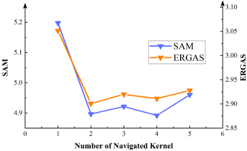
The Number of the Navigated Kernels. In the previous discussion, we set navigated kernel number as 2. In this section, we will justify this setting to see what happens. We have tested the performance of LightNet with different numbers of the navigated kernels. The results are reported in Fig. 5. It is worth to mention that when N is set to 1, the SpanConv degenerates into BSConv. The most obvious improvement is achieved when N increasing from 1 to 2, and metrics become fluctuate when N > 2, which indicates two navigated kernels are enough to construct a qualified kernel space for pansharpening. In addition, during the experiment, we find that the optimized N differs in the different networks and tasks.
The Computational Cost of the Networks. The computational cost of benchmark DL-based methods is presented in Tab. 6. It can be observed that LightNet can achieve the satisfying performance with the fewest computational resource.
The Representation Ability of SpanKernel. In this section, we hook out the weights of LightNet with SpanConv, BSConv, and standard convolution, respectively. And we use ℓ2 distance and Pearson coefficient to measure the difference between the SpanKernel, BlueKernel and the standard convolution kernel. From the results displayed in Tab. 7, the difference of the kernels gradually decrease as the network flows to the end, indicating the correlation become prominent as the networks deepens. In the shallow layer of the network, the difference of SpanKernel and standard convolution kernel are much smaller than that of BlueKernel, illustrating that the kernel space constructed by Spanconv is closer to the standard kernel space. In the other word, campared with BlueKernel, Spanconv can describe richer mapping relationships, thus it has stronger feature representation capabilities.
| Network | Params | FLOPS | MAdd |
|---|---|---|---|
| DRPNN | 1867K | 1.8G | 3.6G |
| MSDCNN | 229K | 936.2M | 1.9G |
| BDPN | 1487K | 3.8G | 7.6G |
| DiCNN | 47K | 191.9M | 382.5M |
| PNN | 104K | 299.9M | 599.1M |
| FusionNet | 79K | 322.7M | 642.4M |
| LightNet | 16K | 67.0M | 126.4M |
| Metrics | ℓ2 distance | Pearson | ||
|---|---|---|---|---|
| Layer Name | BlueKernel | SpanKernel | BlueKernel | SpanKernel |
| head conv1 | 3.040 | 2.870 | 0.032 | 0.068 |
| head conv2 | 0.354 | 0.256 | 0.004 | 0.011 |
| head conv3 | 0.335 | 0.426 | 0.016 | 0.021 |
| belly conv1 | 0.625 | 0.602 | 0.010 | 0.011 |
| belly conv2 | 0.084 | 0.073 | 0.016 | 0.003 |
| belly conv3 | 0.060 | 0.158 | 0.011 | 0.012 |
| belly conv4 | 0.030 | 0.031 | 0.012 | 0.004 |
| tail conv1 | 0.008 | 0.009 | 0.007 | 0.010 |
| tail conv2 | 0.002 | 0.002 | 0.057 | 0.039 |
| tail conv3 | 0.002 | 0.001 | 0.111 | 0.049 |
Limitations. When the kernels have strong independence, the representation ability of our SpanKernel will be limited. As a result, when the kernels display a high degree of dependence fit with the SpanKernel assumption, our technique performs well, consistent with the experimental results.
5 Conclusion
Standard convolution has a high computational cost primarily because the dimension of the convolution kernel is proportional to the channel count of the feature maps. The proposed method introduces a novel convolution operation, SpanConv, that constructs the kernel space by spanning a small number of navigated kernels. A simple end-to-end learning framework, i.e., LightNet, is presented for remote sensing pansharpening task based on the SpanConv. The comparison to the state-of-the-art method demonstrates that our method, to the best of our knowledge, requires the fewest network parameters for pansharpening and achieves superior generalization when achieving competitive outcomes.
Acknowledgments
This research is supported by NSFC (12171072, 61876203, 61702083), Key Projects of Applied Basic Research in Sichuan Province (Grant No. 2020YJ0216), and National Key Research and Development Program of China (Grant No. 2020YFA0714001).
@inproceedings{ijcai2022p118,
  title     = {SpanConv: A New Convolution via Spanning Kernel Space for Lightweight Pansharpening},
  author    = {Chen, Zhi-Xuan and Jin, Cheng and Zhang, Tian-Jing and Wu, Xiao and Deng, Liang-Jian},
  booktitle = {Proceedings of the Thirty-First International Joint Conference on
               Artificial Intelligence, {IJCAI-22}},
  publisher = {International Joint Conferences on Artificial Intelligence Organization},
  editor    = {Luc De Raedt},
  pages     = {841--847},
  year      = {2022},
  month     = {7},
  note      = {Main Track},
  doi       = {10.24963/ijcai.2022/118},
  url       = {https://doi.org/10.24963/ijcai.2022/118},
}
TY - CPAPER TI - SpanConv: A New Convolution via Spanning Kernel Space for Lightweight Pansharpening AU - Chen, Zhi-Xuan AU - Jin, Cheng AU - Zhang, Tian-Jing AU - Wu, Xiao AU - Deng, Liang-Jian T2 - Proceedings of the Thirty-First International Joint Conference on Artificial Intelligence, IJCAI-22 PB - International Joint Conferences on Artificial Intelligence Organization PY - 2022 SP - 841 EP - 847 DO - 10.24963/ijcai.2022/118 UR - https://doi.org/10.24963/ijcai.2022/118 ER -Copied
Machine-readable versions of this paper, for tools and AI agents:





