
Large Neighbourhood Search for Anytime MaxSAT Solving
Proceedings of the Thirty-First International Joint Conference on Artificial Intelligence. Main Track. Pages 1818-1824.
https://doi.org/10.24963/ijcai.2022/253
Keywords
- Constraint Satisfaction and Optimization: Solvers and Tools
- Constraint Satisfaction and Optimization: Satisfiabilty
Abstract
Large Neighbourhood Search (LNS) is an algorithmic framework for optimization problems that can yield good performance in many domains. In this paper, we present a method for applying LNS to improve anytime maximum satisfiability (MaxSAT) solving by introducing a neighbourhood selection policy that shows good empirical performance. We show that our LNS solver can often improve the suboptimal solutions produced by other anytime MaxSAT solvers. When starting with a suboptimal solution of reasonable quality, our approach often finds a better solution than the original anytime solver can achieve. We demonstrate that implementing our LNS solver on top of three different state-of-the-art anytime solvers improves the anytime performance of all three solvers within the standard time limit used in the incomplete tracks of the annual MaxSAT Evaluation.
- [Bacchus et al., 2020a] Fahiem Bacchus, Jeremias Berg, Matti Järvisalo, and Rubens Martins. MaxSAT Evaluation 2020: Solver and Benchmark Descriptions. University of Helsinki, Department of Computer Science, 2020.
- [Bacchus et al., 2020b] Fahiem Bacchus, Matti Järvisalo, and Ruben Martins. Maximum satisfiability. In Handbook of Satisfiability. IOS Press, 2020.
- [Bacchus, 2020] Fahiem Bacchus. Maxhs in the 2020 maxsat evaluation. MaxSAT Evaluation 2020, page 19, 2020.
- [Berg et al., 2019] Jeremias Berg, Emir Demirović, and Pe- ter J Stuckey. Core-boosted linear search for incomplete maxsat. In International Conference on Integration of Constraint Programming, Artificial Intelligence, and Op- erations Research, pages 39-56. Springer, 2019.
- [Berg et al., 2021] Jeremias Berg, Emir Demirović, and Pe- ter J Stuckey. Loandra in the 2020 maxsat evaluation. MaxSAT Evaluation 2021, pages 24-25, 2021.
- [Björdal et al., 2020] Gustav Björdal, Pierre Flener, Justin Pearson, Peter J Stuckey, and Guido Tack. Solving satis- faction problems using large-neighbourhood search. In In- ternational Conference on Principles and Practice of Con- straint Programming, pages 55-71. Springer, 2020.
- [Cai and Lei, 2020] Shaowei Cai and Zhendong Lei. Old techniques in new ways: Clause weighting, unit propaga- tion and hybridization for maximum satisfiability. Artifi- cial Intelligence, 287:103354, 2020.
- [Davies and Bacchus, 2013] Jessica Davies and Fahiem Bac- chus. Exploiting the power of mip solvers in maxsat. In In- ternational conference on theory and applications of sat- isfiability testing, pages 166-181. Springer, 2013.
- [Demirović and Musliu, 2017] Emir Demirović and Nysret Musliu. Maxsat-based large neighborhood search for high school timetabling. Computers & Operations Research, 78:172-180, 2017.
- [Efraimidis and Spirakis, 2006] Pavlos S Efraimidis and Paul G Spirakis. Weighted random sampling with a reservoir. Information Processing Letters, 97(5):181-185, 2006.
- [Lei et al., 2021] Zhendong Lei, Shaowei Cai, Fei Geng, Dongxu Wang, Yongrong Peng, Dongdong Wan, Yip- ing Deng, and Pinyan Lu. Satlike-c: Solver description. MaxSAT Evaluation 2021, page 19, 2021.
- [Li and Manyà, 2009] Chu Min Li and Felip Manyà. MaxSAT, hard and soft constraints. In Handbook of Satis- fiability, pages 613-631. IOS Press, 2009.
- [Lombardi and Schaus, 2014] Michele Lombardi and Pierre Schaus. Cost impact guided lns. In International Con- ference on Integration of Constraint Programming, Arti- ficial Intelligence, and Operations Research, pages 293- 300. Springer, 2014.
- [Nadel, 2019] Alexander Nadel. Anytime weighted maxsat with improved polarity selection and bit-vector optimiza- tion. In 2019 Formal Methods in Computer Aided Design (FMCAD), pages 193-202. IEEE, 2019.
- [Nadel, 2021] Alexander Nadel. Tt-open-wbo-inc-21: an anytime maxsat solver entering mse'21. MaxSAT Eval- uation 2021, pages 21-22, 2021.
- [Parragh and Schmid, 2013] Sophie N Parragh and Verena Schmid. Hybrid column generation and large neighbor- hood search for the dial-a-ride problem. Computers & Op- erations Research, 40(1):490-497, 2013.
- [Perron et al., 2004] Laurent Perron, Paul Shaw, and Vincent Furnon. Propagation guided large neighborhood search. In International Conference on Principles and Practice of Constraint Programming, pages 468-481. Springer, 2004.
- [Ramaswamy and Szeider, 2020] Vaidyanathan Peruvemba Ramaswamy and Stefan Szeider. Maxsat-based postpro- cessing for treedepth. In Helmut Simonis, editor, Princi- ples and Practice of Constraint Programming -26th In- ternational Conference, CP 2020, Louvain-la-Neuve, Bel- gium, September 7-11, 2020, Proceedings, volume 12333 of Lecture Notes in Computer Science, pages 478-495. Springer, 2020.
- [Ropke and Pisinger, 2006] Stefan Ropke and David Pisinger. An adaptive large neighborhood search heuristic for the pickup and delivery problem with time windows. Transportation science, 40(4):455-472, 2006.
- [Shaw, 1998] Paul Shaw. Using constraint programming and local search methods to solve vehicle routing problems. In International conference on principles and practice of constraint programming, pages 417-431. Springer, 1998.
References were extracted automatically from the PDF and may contain errors.
Full text extracted automatically from the PDF; figures, tables and equations may differ. The PDF is the version of record.
1 Introduction
Due to significant advances in maximum satisfiability (MaxSAT) solvers over the past decade, MaxSAT [Li and Many`a, 2009; Bacchus et al., 2020b] has proved itself to be very effective at modelling and solving a range of discrete optimization problems (see [Bacchus et al., 2020b]).
Although the field had previously concentrated on building better complete MaxSAT solvers, i.e., solvers designed to find optimal solutions, in recent years incomplete MaxSAT solvers have become increasingly important. Incomplete solvers do not aim to find optimal solutions, but rather at finding good solutions in less time. In particular, they offer no guarantees on the quality of the solutions they produce, but can be more readily applied in anytime contexts. As the range of applications of MaxSAT solving has grown, some real-world applications, e.g., physical design stage for Computer-Aided Design [Nadel, 2019], high school timetabling [Demirovi´c and Musliu, 2017], etc., have been found to generate problems that are either too large or too difficult for complete solvers to solve to optimality in a timely manner. Hence, as with many real world applications of optimization technology, good, but not necessarily optimal, solutions produced in a reasonable time frame are sought.
Driven by this need, several new ideas, e.g., [Nadel, 2019; Berg et al., 2019; Cai and Lei, 2020] have been developed and proved successful in improving incomplete MaxSAT solvers (as demonstrated in the annual MaxSAT evaluations 1 ) and anytime MaxSAT solving has become an increasingly active area of research in the past few years.
Large Neighbourhood Search (LNS) [Shaw, 1998] is a well-known technique for incomplete solving which has been successfully applied to many optimization problems. The LNS framework involves repeatedly taking an initial solution S, defining a "large" neighbourhood N of S, and then searching N for a better solution than S. Often N is small enough (when compared to the original problem) that it can be exhaustively searched with a complete solver. LNS's effectiveness at finding good solutions is thus determined by the initial solution S and by the selection of the neighbourhood N. In particular, in LNS one aims to select an N that is likely to contain better solutions and that can be effectively searched. Typically, multiple different initial solutions S, and for each S multiple different neighbourhoods N, are tried. LNS has been successfully applied in a number of different domains, showing that it is often possible to develop effective methods for selecting S and N.
Interestingly, although there has been some related work (as discussed below), to the best of our knowledge, LNS has not yet been directly applied in incomplete MaxSAT solving. As pointed out above, LNS offers the possibility of exploiting complete solvers in the context of incomplete solving. Since complete MaxSAT solvers have seen tremendous advances over the past decade, investigating the use of LNS in incomplete MaxSAT solving seems overdue. In this paper we address that gap and develop a neighbourhood selection policy that gives good empirical performance. We find that our approach can often improve the best solution found by other incomplete solvers, but is less effective at turning poor solutions found by those solvers into good solutions. Using this insight we are able to improve the state-of-the-art in incomplete MaxSAT solving by budgeting some time to run our LNS approach on the solutions produced by another incomplete solver. Our method works for both weighted and unweighted instances, and opens the door for investigating other potential ways LNS can be used to improve incomplete MaxSAT solving.
1 https://maxsat-evaluations.github.io/2021
2 Background
A MaxSAT instance F is specified by a weighted CNF. A CNF is a Boolean formula expressed as a conjunction of clauses, where each clause is a disjunction of literals, and each literal is a Boolean variable v or its negation ¬v. The CNF is weighted if every clause has an associated weight that is a positive number or infinity. The soft clauses of the instance F, soft(F), are those with finite weight while those with infinite weight are the hard clauses, hard(F). We use cw to denote the weight of clause c, and we often regard F to be a set of clauses (understood to be a conjunction), and a clause to be a set of literals (understood to be a disjunction).
A total truth assignment π for instance F is a set of literals containing exactly one literal of every variable of F. These literals specify the truth assignments given to the variables: π(v) = true when v ∈ π and π(v) = false when ¬v ∈ π. π satisfies a clause c, written as π |= c, if it contains at least one literal of c. Thus, an empty clause can never be satisfied. The cost of π, cost(π), is the sum of the costs of the clauses it falsifies (i.e., clauses c such that π ̸|= c): cost(π) = ∑c∈{π̸|=c} cw. π is a feasible solution of F if it satisfies every hard clause of F (equivalently if it has finite cost). π is an optimal solution if it is feasible and has lowest cost amongst all feasible solutions. That is, an optimal solution satisfies all hard clauses and falsifies a minimum weight of soft clauses (equivalently, it satisfies a maximimumweight of soft clauses).
Complete and incomplete MaxSAT solvers are required to find feasible solutions. Complete solvers aim to find optimal solutions while incomplete solvers aim to more rapidly find low cost solutions. Anytime MaxSAT solving aims to find the lowest cost solution possible within a given time limit.
A partial truth assignment α is a set of literals with at most one literal of any variable (but not always containing a literal for every variable). The reduction of F by a partial truth assignment α, written as F |α is the process of removing from F all clauses containing a literal of α and then removing from the remaining clauses the negation of all literals in α. The weights of the unremoved clauses are unchanged. This process yields a new instance that is logically equivalent to the formula F ∧ ∧ℓ∈α ℓ. Note, that F |α is smaller than F and is typically easier to solve-especially if α contains a large number of variables. F|α might contain empty clauses due to the second step of the reduction process. If it contains an empty hard clause, it has no feasible solutions. If it contains empty soft clauses, the weight of those soft clauses become part of the cost of every total truth assignment of F|α.
3 Using LNS to Solve MaxSAT Problems
An outline of our approach to using LNS in MaxSAT is given in Algorithm 1. Our approach is parameterized by two auxiliary solvers: (1) an anytime solver AT MaxSlv that provides an initial feasible solution for the instance F and (2) a complete solver C MaxSlv which is able to efficiently and exhaustively search a selected neighbourhood of the current feasible solution. AT MaxSlv is called first to obtain a feasible solution π (a total assignment). In our implementations, we ran AT MaxSlv for a fixed amount of time and used the best solution it found as our initial solution; we experimented with different anytime solvers but always used the same complete solver MaxHS [Bacchus, 2020]. 2
We keep track of the best solution found in the variable best, initializing this to π, the solution returned by AT MaxSlv. The next step is to select a neighbourhood of π than can be searched for a better solution. A common way to do this is to fix some subset of the variables to the value provided in π and leave the remaining variables unfixed. The different assignments to the unfixed variables define the neighbourhood.
In our approach the initial solution π is a total assignment and we can select literals of π to form a partial assignment α whose size is approximately a factor δπ (δ < 1). (Propagation, described below, makes it impossible to select an α with an exact size). The neighbourhood N is thus defined by the different assigments to the variables not appearing in α, while the variables in α remain fixed. It is not difficult to see that N is exactly the set of feasible solutions of F|α. In particular, F |α ≡ F ∧ ∧ℓ∈α ℓ. Hence, β is a feasible solution of F |α iff α ∪ β is a feasible solution of F . Thus, by finding an optimal solution N best of F |α we find the best solution of F that extends α which is α ∪ N best . The benefit of this view is that F|α is simply a new MaxSAT instance. If α is large enough (and thus F |α is small enough), F |α can be efficiently solved to optimality by C MaxSlv .
We refer to the set of literals in the selected partial assignment α as the fixed set, and the process of selecting a fixed set α and then solving F |α as one round of LNS.
Note that for π computed on line 6 of Algorithm 1 we must have that cost(π) ≤ cost(best), unless C MaxSlv on line 3 was interrupted. This is because the truth assignments given in best to the variables of F|α form a feasible solution of F|α. So N best (an optimal solution of F|α) cannot have cost greater than the cost of this feasible solution. That is, at worst C MaxSlv will return an N best such that cost(π) = cost(α ∪ N best) = cost(best). In these cases best will be unchanged and Algorithm 1 will select a different neighbourhood to try to optimize next. When, however, a better solution than best is found, best will be updated and Algorithm 1 will start selecting neighbourhoods of this new solution.
3.1 Neighbourhood Selection
The selection of the neighbourhood N is key to the performance of LNS and several strategies have been explored in other contexts such as [Lombardi and Schaus, 2014]. We tried various methods for selecting N and found that the following popular probabilistic method worked best in our experiments.
The method is simply to randomly select a subset of the literals of the current feasible solution π as the fixed set α, and define N to be the varying assignments to the unfixed vari-
2 In recent MaxSAT evaluations MaxHS has consistently been one of the best complete solvers available. In future work the effect of switching complete solvers will be investigated.
Algorithm 1 Generic LNS algorithm for MaxSAT
Input:
weighted CNF F,
initial solution solver provider AT MaxSlv ,
complete MaxSAT solver C MaxSlv
- 1: π = AT MaxSlv(F) {for fixed time bound}
- 2: best = π
- 3: while time left do
- 4: randomly select α ⊂ π of size ≈ δ|π| {fixed set}
- 6: π = α∪N best
- 5: N best = C MaxSlv(F|α) {interrupt if out of time}
- 7: best = (cost(π) < cost(best)) ?π : best
- 8: return best
ables not in α. The random selection is done using a biased distribution over the literals in which literals we would prefer to keep fixed are given higher probability. Using biased probability distributions to select neighbourhoods has been done in other contexts, such as in [Parragh and Schmid, 2013]. We similarly found that a biased distribution was much more effective than selecting uniformly at random.
The probability distribution that we found to work best was to first assign a weight to each literal ℓ ∈ π equal to the total weight of the soft clauses containing it (these clauses are satisfied by π since π contains ℓ) minus the total cost of falsified soft clauses containing ¬ℓ, where π is used to determine whether or not a clause is falsified. Normalizing these weights yields the required probability distribution over the literals.
Hard clauses were ignored for our weighting, and a slight improvement was obtained by making the weighting exponential. To be precise, in our final implementation the weight ℓw assigned to a literal ℓ ∈ π is
,
and these weights are then normalized to form a distribution over the literals in π, and finally α, a subset of π, is randomly selected from this distribution (selecting without replacement) to form the set of fixed literals. For efficient weighted random sampling, we used the algorithm described in [Efraimidis and Spirakis, 2006].
These weights capture the intuition that we would like to keep literals of π fixed when they help to satisfy a large weight of soft clauses, and when flipping its value satisfies only a small weight of soft clauses. Using exponential weights amplifies the difference between the literals satisfying (falsifying) slightly different weights of soft clauses, but using probabilities and random selection means that literals with high score might not be selected and thus are allowed to vary in the selected neighbourhood.
Propagation has been used in other contexts when selecting neighbourhoods for LNS [Perron et al., 2004], and we found it to be beneficial in our approach. In particular, as we randomly select each literal ℓ to be fixed, we incrementally add ℓ to hard(F) and perform unit propagation on hard(F). All
Algorithm 2 Neighbourhood selection policy
Input:
weighted CNF F, current feasible solution π, δ desired size of fixed set
- 1: α = ∅ // initialize fixset to empty
- 3: for each c ∈ soft(F) do
- 2: for each l ∈ π: lw = 0
- 4: if π |= c then
- 6: else
- 5: for each l ∈ c: lw = lw + cw
- 7: for each l ∈ c: (¬l)w = (¬l)w - cw
- 9: for each l ∈ π: prob(l) = 2lw ∑l∈π 2lw
- 8: // Note that if π ̸|= c then l ∈ c → ¬l ∈ π
- 10: hards = hard(F)
- 11: while size(α) < δ|π| do
- 13: // add l to hards and unit prop
- 12: select l ∈ π randomly with prob(l).
- 14: hards = UP(hards ∪ (l))
- 15: α = all units in hards // Note the units of hards includes all selected literals // and all of their unit implications
- 16: return α // Final selected fixed set
unit implied literals are forced by the hard clauses to be fixed in all feasible solutions containing the previously randomly selected set of fixed literals. Hence, we add these implied literals to the fixed set α and continue to randomly select literals for α amongst the remaining literals of π not yet in α, stopping when α reaches or exceeds the desired size, δ|π| (δ < 1). (Since we cannot predict how many unit implicants will be added to α we cannot select an exactly sized α.) Note that since π is a feasible solution satisfying hard(F) and all selected literals are in π, all unit implied literals u found in this way must also be in π. Hence, we still have that α ⊂ π. One benefit of propagation is that it allows better control over the size of the unfixed neighbourbood N. An unpropagated α might have many implied literals not in α, and each such literal reduces the possible number of feasible solutions in N since these literals are implicitly fixed in N.
We start with a fixed set α of size about 80% of the total number of variables in the problem, i.e., with δ = 0.8. After ten consecutive rounds of LNS where no new best solution is found, we reduce α's size by reducing δ by 0.1. We decided to start with a small neighbourhood (a large fixed set) because small neighbourhoods will usually be easier to solve with C MaxSlv. Notice that once δ gets to 0.1 and we encounter ten consecutive rounds with no new best solution, δ will be set to 0 and the entire problem will be solved by C MaxSlv optimally. In our experiments this very rarely happened (less than 0.5% of all instances). We also found that dynamically decreasing δ worked considerably better than using a fixed value. For clarity, our final neighbourhood selection policy is given in Algorithm 2.
One other minor improvement not shown in Algorithm 2 is that the selected fixed set α generally falsifies some soft clauses (all soft clauses c with l ∈ c → ¬l ∈ α). Let cost(α) denote the sum of the costs of the clauses falsified by α. (Note that since α is a partial assignment some clauses are neither satisfied nor falsified by α). This means in any round of LNS in Algorithm 1 the cost of the best solution found in each neighbourhood is at least cost(α), i.e., cost(α∪N best) ≥ cost(α). Hence, if cost(α) ≥ cost(best) there is no point in searching the neighbourhood defined by α-that neighbourhood cannot yield a better solution. Hence, we check cost(α) and immediately fail that round without calling C MaxSlv(F|α) if cost(α) ≥ cost(best). It is also possible to reject α when its cost is too close to cost(best), but exploring this option is left for future work.
It would perhaps be more accurate to keep a list of soft clauses and remove those that are satisfied by each literal as that literal is added into the fixed set, i.e., after adding a literal l to the fixed set, we would re-compute the preference weighting for all remaining literals using the updated soft clauses list. However, this is more costly requiring multiple passes of the soft clauses during the neighbourhood selection process, whereas our neighbourhood selection process requires just one pass. In our experiments, doing only one pass of the soft clauses seemed to work better so we decided to proceed with that.
An alternative approach of neighbourhood selection would be to select some subset of the soft clauses satisfied in the initial solution to be a fixed set. These soft clauses would then be treated as hard clauses (i.e., we would force these soft clauses to be satisfied), and C MaxSlv would find an optimal way to satisfy the remaining unfixed soft clauses. We experimented with this and found it was not quite as good as fixing literals, so we decided to focus on literal fixing for the rest of our implementations.
4 Experiments and Results
All of our experiments were run on 2.7GHz Intel cores with 300 second CPU time and 16GB memory limits. 3 The benchmarks we used for the first two experiments were the 253 weighted and 262 unweighted instances from the Incomplete Tracks of the 2020 MaxSAT Evaluation [Bacchus et al., 2020a] (we used the 2020 benchmarks instead of 2021 because there are more total instances in the 2020 benchmarks). In order to avoid overfitting, we did all tuning of our neighbourhood selection policy on the instances from the 2018 and 2019 MaxSAT Evaluations before settling on the policy described in Section 3.1. We implemented our LNS algorithm as described in Section 3 using MaxHS [Bacchus, 2020] as the complete solver C MaxSlv . To measure how effective our approach was at finding good solutions, we used the same scoring system as used in the MaxSAT evaluations. In particular, the score a solver S achieves on an instance i is score(S, i) = bki+1 sci+1 , where sci is the cost of the best solution found by S for instance i and bki is the cost of the best known solution for instance i. The values bki were supplied by the MaxSAT evaluation. On an instance i a score of 1 indicates that S found a solution of cost equal to the best known, and a score of 0 indicates that S was unable to find any feasible solution (in this case sci = ∞). The score of S on a set of instances I is simply its average score over these instances: score(S, I) = ∑i∈I score(S,i) |I | .
3 The MaxSAT evaluations also test a time out of 60 seconds, and we experimented with that time out as well. However our approach involves many calls to C MaxSlv in the main loop of LNS and in our current implementation these calls are not optimized for incrementality. In particular, each call to C MaxSlv requires processing the input instance from scratch and re-initializing the solver with a new reduced instance. For the many large instances appearing in the evaluation this imposed an overhead that significantly impacted the shorter 60 second runs. So much so that we did not find LNS to be effective in the 60 second context. There are a number of ways a more sophisticated implementation could reduce this overhead, so we left making LNS effective in this shorter time frame as future work. In general, properly addressing this issue requires improved techniques for incremental MaxSat solving which is an important area for future research.
Our first experiment is designed to evaluate how effective LNS is at improving feasible solutions, and to compare this to how effective a representative state-of-the-art anytime solver is at the same task. In particular, when an anytime solver AT MaxSlv is run on an instance it will emit a sequence of monotonically improving solutions (decreasing solution costs) over its 300s run. If we take a solution π emitted at time t (measured in seconds) we can use this sequence to determine the best solution π′ emitted at time t + ∆ for any interval ∆. (π′ might be the same as π if no better solution has been found ∆ seconds after π was found). We can then measure the improvement in solution cost achieved from solution π, cost(π) - cost(π′ ), as a function of time ∆. We can do the same for the LNS solver by giving it π as its initial solution.
We chose TT-Open-WBO [Nadel, 2021], one of the best incomplete solvers in recent MaxSAT evaluations, as the representative state-of-the-art anytime solver to compare LNS "rate of improvement" with. 4
We ran TT-Open-WBO on each instance from the 2020 MaxSAT incomplete solver evaluation for 600s, combining the weighted and unweighted instances to obtain 515 instances. 5 For each instance we stored the timestamped sequence of solutions TT-Open-WBO emitted. This allowed us to use any solution emitted by TT-Open-WBO within the first 300s and still have a full 300s "future" for that solution. We took all solutions-instances pairs where the solution was emitted by TT-Open-WBO in the first 300 seconds and further filtered them to control their total number. In particular, if multiple solutions for that instance were found in the same 5-second interval, only the best one was kept. We then ran our LNS algorithm for 300s on each of the these solution-instance pairs. We similarly recorded the sequence of solutions emitted by LNS for each solution-instance pair over its 300s run. This gave us a set of solution-instance pairs along with a 300s future evolution of those solutions in TT-Open-WBO and in LNS.
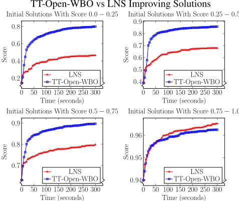
To compare the rate of improvement of TT-Open-WBO with that of LNS, we split the solutions into four buckets based on solution quality. The reason for separating the solutions is that poor solutions typically can be improved at a much faster rate by either solver than good solutions. The first bucket had solutions with a score between 0.0 and 0.25, the second with scores between 0.25 and 0.5, the third with scores between 0.5 and 0.75, and the fourth with scores between 0.75 and 1.0. Then, for each bucket of solutions, we kept only one randomly picked solution per instance, since some instances contributed multiple solutions to the same bucket which would bias the results towards those instances. This left the first bucket with 75 solutions, the second bucket with 109 solutions, the third bucket with 136 solutions, and the fourth bucket with 453 solutions. We plot in Figure 1 the average score obtained over all solution-instance pairs in the bucket and how it increased with time as LNS worked on them, compared to the average score that TT-Open-WBO achieved over time for the same solution-instance pairs.
4 Other incomplete solvers gave similar results.
5 For this experiment we were not interested in distinguishing these two cases.
We can observe that LNS is able to achieve a good improvement of the solutions in all buckets. In fact, for the first 5-10 seconds it is able to improve the solution quality faster (as fast for the 0.5-0.75 solutions) than TT-OpenWBO. However, for the lower quality solutions (those with scores < 0.75), its rate of improvement quickly diminishes and its final level of improvement was considerably worse than TT-Open-WBO. This makes intuitive sense. LNS intensely searches neighbourhoods close to the solution it starts with, and it can take it a long time to move far away from that solution. TT-Open-WBO on the other hand has much more mobility in the search space and is able to move away from bad initial solutions more quickly.
When we examine the highest quality solutions, those in the 0.75-1 bucket, we see that TT-Open-WBO can achieve some improvement to these solution. But its rate of improvement is no better than LNS. More importantly, its final level of improvement is worse than LNS. We conjecture, that for these higher quality solutions there are not as many better solutions, and it is not as easy for TT-Open-WBO to find them. Whereas LNS, by searching more systematically, is more effective at finding these more sparse better solutions.
This data suggests that a promising way to use LNS is to ensure that the anytime solver has enough time to produce a higher quality solution and then use LNS to improve that solution. In our next experiment we tried giving the anytime solver various fixed amounts of time (i.e., running it for the same amount of time on each instance) before finishing up with using our LNS solver. An alternative that would be worth investigating in future work would be to try to detect when the anytime solver is plateauing in its ability to improve the solution and invoke the LNS solver at that point.
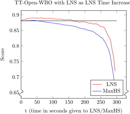
Our second experiment used the same data as experiment one. As mentioned above it involved running TT-Open-WBO for some amount of time, before switching to our LNS solver for the remaining amount of time and finally outputing the best solution found. In Figure 2, we show the total score achieved when taking the best solution for each instance emitted by TT-Open-WBO within 300-t seconds and then allowing our LNS solver t seconds to improve those solutions (for different values of t). Note, that when t = 0 we obtain the baseline performance of TT-Open-WBO, and this baseline is indicated in Figure 2 by the horizontal dashed line. Figure 2 clearly shows that stopping TT-Open-WBO early and running LNS for some amount of time resulted in a performance gain up until a threshold of about 50 seconds after which the performance starts to decline.
Since the LNS solver is based on MaxHS, which uses a different MaxSAT algorithm [Davies and Bacchus, 2013], some of the performance gain obtained by switching from TT-Open-WBO to LNS could be simply because we are using two different solvers and taking the best solution computed by either of them. This is known as the portfolio effect. To demonstrate that the performance gain is not solely from the portfolio effect, we also show in Figure 2 the score achieved by running TT-Open-WBO for 300 - t seconds and then running plain MaxHS for t seconds. Note that MaxHS also outputs intermediate solutions, so in cases where MaxHS can not solve optimally, we take the best solution it output and use that as its solution. We can see that using LNS dominates using MaxHS for all values of t, indicating the performance gain is not solely due to a portfolio effect.
For the last set of experiments, we try to improve the performance of three of the best performing anytime MaxSAT solvers from the 2020 and 2021 MaxSAT evaluations: TTOpen-WBO, Loandra [Berg et al., 2021], and satlike [Lei et al., 2021]. Loandra is a SAT-solver based MaxSAT solver, while TT-Open-WBO and satlike use a combination of SAT-solving and local-search. We implemented three solvers, LNS-TT-Open-WBO 6 , LNS-satlike, and LNSLoandra, which ran the corresponding anytime MaxSAT solver for 250 seconds and then used our LNS solver to improve the best solution they found for the final 50 seconds. The 50 second limit for LNS was based on the data shown in Figure 2. We also ran the base solvers TT-Open-WBO, satlike, and Loandra for 300 seconds each in order to compare them to the LNS hybrid versions. For this last set of experiments, we used the union of all weighted and unweighted instances from the 2020 and 2021 MaxSAT evaluations. After removing duplicates, this left 352 weighted instances and 374 unweighted instances for a total of 726 instances. The results are given in Table 1.
6 Source code can be found at https://github.com/rgh000/ MaxSAT LNS.
For both the weighted and unweighted instances, the total scores obtained by the LNS versions were an improvement over the baseline for all three solvers. Although the improvements may appear small, even modest improvements are difficult to achieve on MaxSAT competition benchmarks. To give some context, in the four tracks of the 2020 MaxSAT Evaluation, the average difference between the winning solver and the runner-up was 0.0075 in average score, and in 2021 it was 0.0178. The LNS solvers are also finding better solutions than any other solver had previously found. In total, the three LNS solvers was were able to improve the best known solution for 55 of the 515 total instances from 2020 and 40 of the 306 total instances from 2021. On average in these cases the best known solution was improved by 3.7% for 2020 instances and 4.8% for 2021 instances; the maximum improvement we saw to a previously best known solution was 85.7%. These results make it clear that budgeting some time for LNS to run on the best solution obtained from any of these anytime solvers is a good strategy to improve their performance (on these benchmark instances). Since these three anytime solvers were the best performing solvers in the evaluation, we can see that our approach improves the state-of-the-art.
5 RelatedWork
In [Demirovi´c and Musliu, 2017] an LNS method that uses a MaxSAT solver as part of its workflow was used to improve initial solutions for high school timetabling problems, but not used to solve MaxSAT problems directly. In finding initial solutions to these high school timetabling problems, domainspecific information was taken advantage of rather than converting the whole problem directly into MaxSAT from the start.
| Solver | Weighted | Unweighted | Total |
|---|---|---|---|
| TT-Open-WBO | .855 | .853 | .854 |
| LNS-TT-Open-WBO | .866 | .864 | .865 |
| satlike | .836 | .850 | .843 |
| LNS-satlike | .855 | .867 | .861 |
| Loandra | .835 | .825 | .830 |
| LNS-Loandra | .848 | .845 | .846 |
In [Ramaswamy and Szeider, 2020] a MaxSAT solver is used to make local improvements to treewidth decompositions. Their work is similar to using LNS except that the neighbourhood is defined by the structure of the graph they are working with.
In [Bj¨ordal et al., 2020] it was shown how LNS can be used to help solve very difficult satisfiability problems, but LNS was not used to solve MaxSAT problems. It would be interesting to see if some of the ideas that were successful in solving very difficult satisfiability problems with LNS could be adapted to solve MaxSAT problems.
In none of these works, however, do we find a direct application of LNS to MaxSAT solving.
6 FutureWork
The approach to using LNS we have described uses LNS once to improve a feasible solution produced by another anytime solver. However, with more implementation work a tighter integration between the solvers could be achieved. In particular, our results indicate that LNS can often more rapidly improve even a poor solution in the first 5 to 10 seconds. Potentially this could be exploited in an anytime solver, by having it invoke LNS for a brief time to improve each solution it finds. This idea has even more potential if ways could be found for the anytime solver to take advantage of the LNS improved solution, e.g., by adjusting its search for the next better solution. It is an interesting research project to find effective ways of accomplishing this.
Another area for future work is further development of incremental MaxSAT solving. the LNS solver is called many times and building an incremental framework to allow reusing the work of previous calls to C MaxSlv (e.g., previously discovered cores or learnt clauses) could result in a speedup.
Finally, it is known that LNS can get stuck exploring a local part of the solution space when the neighbourhood selection policy does not allow for enough diversity. We observe from our experiments that this is probably what is happening to our neighbourhood selection policy and one way to combat this might be to use some strategies from the literature that have worked in other contexts, such as adaptive large neighbourhood search [Ropke and Pisinger, 2006].
7 Conclusion
We have shown that running LNS for a small amount of time can improve suboptimal MaxSAT solutions faster than those solvers can improve their own respective solutions. By implementing our LNS algorithm to operate on the best solution from the anytime solver, we were able to improve the anytime performance of three of the best performing anytime solvers on both the weighted and unweighted incomplete benchmarks from the MaxSAT Evaluation competitions. We believe that using LNS to find better solutions faster is a good addition to anytime MaxSAT solving and deserves further exploration. It is possible that by fine-tuning the parameters of our algorithm or by allowing LNS to operate multiple times on different solutions from the base solver that even further improvements could be achieved.
@inproceedings{ijcai2022p253,
  title     = {Large Neighbourhood Search for Anytime MaxSAT Solving},
  author    = {Hickey, Randy and Bacchus, Fahiem},
  booktitle = {Proceedings of the Thirty-First International Joint Conference on
               Artificial Intelligence, {IJCAI-22}},
  publisher = {International Joint Conferences on Artificial Intelligence Organization},
  editor    = {Luc De Raedt},
  pages     = {1818--1824},
  year      = {2022},
  month     = {7},
  note      = {Main Track},
  doi       = {10.24963/ijcai.2022/253},
  url       = {https://doi.org/10.24963/ijcai.2022/253},
}
TY - CPAPER TI - Large Neighbourhood Search for Anytime MaxSAT Solving AU - Hickey, Randy AU - Bacchus, Fahiem T2 - Proceedings of the Thirty-First International Joint Conference on Artificial Intelligence, IJCAI-22 PB - International Joint Conferences on Artificial Intelligence Organization PY - 2022 SP - 1818 EP - 1824 DO - 10.24963/ijcai.2022/253 UR - https://doi.org/10.24963/ijcai.2022/253 ER -Copied
Machine-readable versions of this paper, for tools and AI agents:





