
Encoding Probabilistic Graphical Models into Stochastic Boolean Satisfiability
Proceedings of the Thirty-First International Joint Conference on Artificial Intelligence. Main Track. Pages 1834-1842.
https://doi.org/10.24963/ijcai.2022/255
Keywords
- Constraint Satisfaction and Optimization: Modeling
- Constraint Satisfaction and Optimization: Constraint Satisfaction
- Constraint Satisfaction and Optimization: Solvers and Tools
- Constraint Satisfaction and Optimization: Satisfiabilty
- Constraint Satisfaction and Optimization: Applications
Abstract
Statistical inference is a powerful technique in various applications. Although many statistical inference tools are available, answering inference queries involving complex quantification structures remains challenging. Recently, solvers for Stochastic Boolean Satisfiability (SSAT), a powerful formalism allowing concise encodings of PSPACE decision problems under uncertainty, are under active development and applied in more and more applications. In this work, we exploit SSAT solvers for the inference of Probabilistic Graphical Models (PGMs), an essential representation for probabilistic reasoning. Specifically, we develop encoding methods to systematically convert PGM inference problems into SSAT formulas for effective solving. Experimental results demonstrate that, by using our encoding, SSAT-based solving can complement existing PGM tools, especially in answering complex queries.
- [Bart et al., 2016] Anicet Bart, Frédéric Koriche, Jean-Marie Lagniez, and Pierre Marquis. An improved CNF encoding scheme for probabilistic inference. In European Confer- ence on Artificial Intelligence, pages 613-621, 2016.
- [Chavira and Darwiche, 2008] Mark Chavira and Adnan Darwiche. On probabilistic inference by weighted model counting. Artificial Intelligence, 172(6):772-799, 2008.
- [Chen et al., 2013] Suming Jeremiah Chen, Arthur Choi, and Adnan Darwiche. An exact algorithm for computing the same-decision probability. In International Joint Confer- ence on Artificial Intelligence, pages 2525-2531, 2013. IJCAI
- [Chen et al., 2021] Pei-Wei Chen, Yu-Ching Huang, and Jie- Hong R. Jiang. A sharp leap from quantified boolean for- mula to stochastic boolean satisfiability solving. In AAAI Conference on Artificial Intelligence, pages 3697-3706, 2021.
- [Choi et al., 2012] Arthur Choi, Yexiang Xue, and Adnan Darwiche. Same-decision probability: A confidence mea- sure for threshold-based decisions. International Journal of Approximate Reasoning, 53(9):1415-1428, 2012.
- [Dechter, 2000] Rina Dechter. A new perspective on algo- rithms for optimizing policies under uncertainty. In In- ternational Conference on Artificial Intelligence Planning Systems (AIPS), pages 72-81, 2000.
- [Fremont et al., 2017] Daniel J Fremont, Markus N Rabe, and Sanjit A Seshia. Maximum model counting. In AAAI Conference on Artificial Intelligence, pages 3885-3892, 2017.
- [Freudenthal and Karamcheti, 2003] Eric Freudenthal and Vijay Karamcheti. QTM: Trust management with quan- tified stochastic attributes. NYU Computer Science Tech- nical Report TR 2003-848, 2003.
- [Kask et al., 2005] Kalev Kask, Rina Dechter, Javier Lar- rosa, and Avi Dechter. Unifying tree decompositions for reasoning in graphical models. Artificial Intelligence, 166(1-2):165-193, 2005.
- [Kjaerulff and Madsen, 2013] Uffe B. Kjaerulff and An- ders L. Madsen. Bayesian Networks and Influence Dia- grams: A Guide to Construction and Analysis. Springer, 2013.
- [Koller and Friedman, 2009] Daphne Koller and Nir Fried- man. Probabilistic Graphical Models: Principles and Techniques. The MIT Press, 2009.
- [Lee and Jiang, 2018] Nian-Ze Lee and Jie-Hong R Jiang. Towards formal evaluation and verification of probabilis- tic design. IEEE Transactions on Computers, 67(8):1202- 1216, 2018.
- [Lee et al., 2017] Nian-Ze Lee, Yen-Shi Wang, and Jie- Hong R. Jiang. Solving stochastic Boolean satisfiabil- ity under random-exist quantification. In International Joint Conference on Artificial Intelligence, pages 688- 694, 2017. IJCAI
- [Lee et al., 2018] Nian-Ze Lee, Yen-Shi Wang, and Jie- Hong R Jiang. Solving exist-random quantified stochastic Boolean satisfiability via clause selection. In International Joint Conference on Artificial Intelligence, pages 1339- 1345, 2018. IJCAI
- [Lee et al., 2021] Junkyu Lee, Radu Marinescu, and Rina Dechter. Submodel decomposition bounds for influence diagrams. In AAAI Conference on Artificial Intelligence, pages 12147-12157, 2021.
- [Littman et al., 2001] Michael L Littman, Stephen M Majer- cik, and Toniann Pitassi. Stochastic Boolean satisfiability. Journal of Automated Reasoning, 27(3):251-296, 2001.
- [Littman, 1997] Michael L. Littman. Probabilistic proposi- tional planning: Representations and complexity. In Na- tional Conference on Artificial Intelligence, pages 748- 754, 1997.
- [Littman, 1999] Michael L. Littman. Initial experiments in stochastic satisfiability. In National Conference on Artifi- cial Intelligence, pages 667--672, 1999.
- [Majercik and Boots, 2005] Stephen M. Majercik and Byron Boots. DC-SSAT: A divide-and-conquer approach to solv- ing stochastic satisfiability problems efficiently. In Na- tional Conference on Artificial Intelligence, pages 416- 422, 2005.
- [Majercik and Littman, 1998] Stephen M Majercik and Michael L Littman. MAXPLAN: A new approach to probabilistic planning. In International Conference on Artificial Intelligence Planning Systems, volume 98, pages 86-93, 1998.
- [Majercik and Littman, 2003] Stephen M. Majercik and Michael L. Littman. Contingent planning under uncer- tainty via stochastic satisfiability. Artificial Intelligence, 147(1-2):119-162, 2003.
- [Marinescu et al., 2018] Radu Marinescu, Junkyu Lee, Rina Dechter, and Alexander T. Ihler. AND/OR search for marginal MAP. Journal of Artificial Intelligence Research, 63:875-921, 2018.
- [Oztok et al., 2016] Umut Oztok, Arthur Choi, and Adnan Darwiche. Solving pp pp -complete problems using knowl- edge compilation. In Principles of Knowledge Represen- tation and Reasoning, pages 94-103, 2016.
- [Papadimitriou, 1985] Christos Papadimitriou. Games Against Nature. Journal of Computer and System Sci- ences, 31(2):288-301, 1985.
- [Park and Darwiche, 2004] James D. Park and Adnan Dar- wiche. Complexity results and approximation strategies for MAP explanations. Journal of Artificial Intelligence Research, 21:101-133, 2004.
- [Roth, 1996] Dan Roth. On the hardness of approximate rea- soning. Artificial Intelligence, 82(1):273-302, 1996.
- [Sang et al., 2005] Tian Sang, Paul Beame, and Henry A. Kautz. Performing bayesian inference by weighted model counting. In National Conference on Artificial Intelli- gence, pages 475-482, 2005.
- [Shachter, 1986] Ross D. Shachter. Evaluating influence di- agrams. Oper. Res., 34(6):871-882, 1986.
References were extracted automatically from the PDF and may contain errors.
Full text extracted automatically from the PDF; figures, tables and equations may differ. The PDF is the version of record.
1 Introduction
Stochastic Boolean Satisfiability (SSAT) is a formalism, proposed in [Papadimitriou, 1985], to model decision problems under uncertainty, a.k.a, games against nature. It generalizes quantified Boolean satisfiability (QSAT) by allowing randomized quantification over Boolean variables. This generalization makes SSAT suitable for probabilistic decision making, e.g., in probabilistic planning [Littman et al., 2001; Majercik and Littman, 1998; Majercik and Littman, 2003], trust management [Freudenthal and Karamcheti, 2003], belief network inference [Littman et al., 2001], and probabilistic equivalence checking [Lee and Jiang, 2018]. Due to the general applicability of SSAT and the recent advancements in SAT and QBF solving, the decision procedure for solving SSAT formulas is under active research and development. To date, there are general solvers, e.g., ZANDER [Majercik and Littman, 2003], DC-SSAT [Majercik and Boots, 2005], ClauSSat [Chen et al., 2021], and special solvers, e.g., MAXPLAN [Majercik and Littman, 1998], reSSAT [Lee et al., 2017], erSSAT [Lee et al., 2018], MaxCount [Fremont et al., 2017], available.
In a stochastic system, the joint probability distribution of its random variables may often be characterized with conditional probabilities and represented with a probabilistic graphical model (PGM) [Koller and Friedman, 2009]. Nevertheless, conditional probabilities cannot be explicitly expressed in the SSAT formalism. Although there are efforts encoding conditional probabilities of Bayesian network inference into propositional clauses, e.g., [Littman, 1999; Sang et al., 2005; Chavira and Darwiche, 2008; Bart et al., 2016], they are limited to #P- or PP-complete problems [Roth, 1996] under the weighted model counting formulation, a special case of SSAT without quantifier alternations. In principle, SSAT, a PSPACE-complete problem, is generally applicable to pervasive tasks in PSPACE. In this work, we aim to apply SSAT for statistical inferences involving complex quantification structures on a PGM.
In particular, we consider statistical queries, including the NPPP-complete maximum a posteriori (MAP) query on Bayesian networks [Park and Darwiche, 2004], the PPPPcomplete same-decision probability (SDP) query on Bayesian networks [Choi et al., 2012], and the PSPACE-complete maximum expected utility (MEU) query on influence diagrams [Littman et al., 2001]. Essentially, we encode these queries into (extended) SSAT formulas for evaluation. Experimental results demonstrate that the SSAT-based method is comparable and complementary to the state-of-the-art PGM algorithms for MAP problems. Furthermore, for the more complex SDP query on Bayesian networks and MEU query on influence diagrams, our method is more scalable than PGM solvers. It uniquely resolves several instances not attainable by PGM solvers.
The rest of the paper is organized as follows. Section 2 provides the preliminaries for essential backgrounds. Section 3 presents the encoding of MAP and SDP queries on Bayesian networks; Section 4 gives the encoding of MEU queries on influence diagrams. Some implementation issues are addressed in Section 5. After experimental evaluation is detailed in Section 6, related work is discussed in Section 7. Finally, Section 8 draws the conclusions.
2 Preliminaries
For Boolean connectives in a Boolean expression, we denote conjunction by "∧", implication by "→", biconditional by
"↔", and negation by "¬". A Boolean variable takes on a value in the Boolean domain B = {⊥,⊤}, for either TRUE ⊤ or FALSE ⊥. A literal is a variable x or a negation of a variable ¬x. A clause is a disjunction of literals, and a cube is a conjunction of literals. We alternatively view a clause or cube as a set of literals. A conjunctive normal form (CNF) formula is a conjunction of clauses.
An assignment α over a set of variables X is a mapping α : X → B. We alternatively treat α as a cube consisting of literals {l | l = x for α(x) = ⊤, l = ¬x for α(x) = ⊥}. The set of assignments to variables X is denoted as [[X]]. The cardinality of a set X is denoted as |X|.
A Boolean formula over variables X is satisfiable if it is TRUE under some assignment to X. Otherwise, it is unsatisfiable. The Boolean satisfiability (SAT) problem asks whether a given CNF formula is satisfiable.
2.1 Stochastic Boolean Satisfiability
An SSAT formula Φ in the prenex form can be expressed by
where Qixi with Qi ∈ {∃, R pi } indicates variable xi being existentially quantified for Qi = ∃ or randomly quantified for Qi = R pi , the sequence Q1x1, . . . ,Qnxn is called the prefix, and ϕ is a quantifier-free formula over variables {x1, . . . , xn} referred to as the matrix. The randomized quantification R pi xi specifies xi being a randomized variable with probability Pr[xi = ⊤] = pi. We assume that ϕ is in CNF. For variable xi, its quantification level equals the number of alternations between existential and randomized quantifiers from Q1 to Qi plus 1. The quantification level of an SSAT formula is the maximum among the quantification levels of all variables.
Given an SSAT formula Φ, the semantics of Φ is interpreted as the satisfaction probability Pr[Φ] evaluated recursively as follows. Let v be the outermost variable in the prefix of Φ.
- Pr[⊤] = 1,
- Pr[⊥] = 0,
- Pr[Φ] = max{Pr[Φ|¬v],Pr[Φ|v]}, for v being existentially quantified,
- Pr[Φ] = (1-p) ×Pr[Φ|¬v] +p×Pr[Φ|v], for v being randomly quantified by R p ,
where Φ|v (respectively Φ|¬v) is the SSAT formula derived from Φ by assigning v to ⊤ (respectively ⊥) in its matrix and removing the quantification of v from its prefix.
2.2 Bayesian Network
A Bayesian network (BN), a special case of the probabilistic graphical model [Koller and Friedman, 2009], is a directed acyclic graph (DAG) GBN = (V,E), where V is a set of vertices corresponding to random variables X = {Xv | v ∈ V } and E ⊆ V × V is a set of directed edges signifying conditional dependencies among the variables. A vertex in a BN is referred to as a chance node. For each vertex v ∈ V , the random variable Xv can take on values in its domain set Sv. The probability distribution function Pr[Xv|Xu1 , . . . , Xuk ], or denoted Pr[Xv|Xparents(v)] for brevity, of Xv under all possible valuations of the random variables of its parent vertices parents(v) = {u1, . . . , uk} is specified by a conditional probability table (CPT). The CPT of vertex v with parents(v) = {u1, . . . , uk} is of dimension (|Su1 ||Su2 | · · · |Suk |)×|Sv| such that its rows are indexed by the combinations of values in the product domain set Su1 × Su2 × . . . ×Suk and its columns are indexed by the values in Sv. The entry at the ith column (with Xv = svi ) and j th row (with Xu1 = su1 j1 , . . . , Xuk = suk jk ) in the CPT corresponds to the probability Pr[Xv = svi |Xu1 = su1 j1 , . . . ,Xuk = suk jk ]. Hence, the summation of the probability values of each row of a CPT equals 1. For brevity, in the sequel we omit specifying the underlying random variables in the conditional probability Pr[Xv = svi |Xu1 = su1 j1 , . . . ,Xuk = suk jk ] and simply write Pr[svi |su1 j1 , . . . , suk jk ].
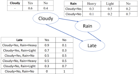
Figure 1 shows a Bayesian network example, which relates the weather conditions and the lateness status of a student attending a class. Node Cloudy gives the weather condition at the student's place; node Rain, conditioned on Cloudy, specifies the weather condition at the school; node Late, conditioned on Cloudy and Rain, presents the lateness status of the student. Each node is associated with a CPT.
In this work, we consider the inference queries of maximum a posterior (MAP) and same-decision probability (SDP) on Bayesian networks.
The MAP query asks to find the most probable combination of values of a set of variables in a BN. The fact that some random variables take on their values is called an evidence. Given the evidence e of the variables XE ⊆ X and a set of variables XY ⊆ X which is disjoint with XE, the MAP is defined by
where y is the combination of values which the variables in XY take on.
Consider the Bayesian network example in Figure 1. Given the evidence that the student is not late for a class, we may ask which one of the cloudy and not cloudy situations is the most probable. Formally, the MAP can be expressed by
The SDP, proposed in [Choi et al., 2012], corresponds to a confidence measure for threshold-based decisions in a BN. Given the evidence e of the variables XE ⊆ X, a hypothesis d of a variable Xd ∈ X, a threshold T, and a set of unobserved variables XH ⊆ X. Suppose a decision is made by checking Pr[d|e] ≥ T . The variable Xd is called the decision variable. The SDP in this scenario is
where h is a combination of values of XH and
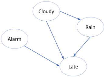
To illustrate the SDP problem, consider the Bayesian network shown in Figure 2, which adds one more factor Alarm to the student's lateness. A teacher would like to decide whether to visit the student's parents depending on the weather condition at the student's place, and would judge the probability of cloudy weather by the student's lateness. If the probability of cloudy weather is greater than 0.5, the teacher will postpone the visit. Given that the student is not late, the teacher can calculate the probability of cloudy weather by Pr[Cloudy|Late = No]. Assume Alarm is an unobserved variable. The SDP problem may ask the probability for the same decision of the visit under all status of the alarm, which is
where Prt(Alarm) is defined as Pr[Cloudy|Late = No, Alarm] ≥ 0.5.
2.3 Influence Diagram
An influence diagram (ID) [Kjaerulff and Madsen, 2013], generalized from a Bayesian network, can also be represented by a DAG GID = (V,E). There are three types of vertices forming a partition on V , including chance nodes VC, same as those in a Bayesian network, decision nodes VD, and utility nodes VU. A chance node v ∈ VC is associated with a chance variable Xv and a CPT specifying the probability distribution function Pr[Xv|Xparents(v)]; a decision node v ∈ VD is associated with a decision variable Dv; a utility node v ∈ VU is associated with a utility function utilv : Su1 ×. . .×Suk → R, for parents(v) = {u1, . . . , uk}, that maps the combinations of values of its parent vertices to a real number. In an influence diagram, only chance nodes and decision nodes can have directed edges pointing to other vertices. The edges can be categorized into three types: An edge e = (u, v) ∈ V ×VC indicates the influence of u in the conditional probability of the chance node v; an edge e = (u, v) ∈ V × VD indicates that the value of u should be known before making a decision at the decision node v; an edge e = (u, v) ∈ V ×VU indicates that u is an input to the utility function of the utility node v.
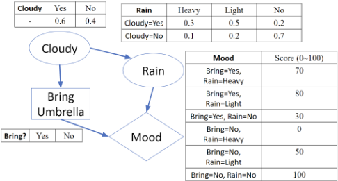
Figure 3: An influence diagram example about weather conditions and the decision to bring an umbrella or not.
For decision-making in an influence diagram, the decisions have to be made conforming to the topological order of the decision nodes. A decision policy specifies the choices of each decision node under all possible combinations of values of its parent nodes. An expected utility (EU) is the expected value of the utility under a decision policy. A common decision-making problem on an influence diagram asks to find the best decision policy to attain the maximum expected utility (MEU).
An influence diagram example is shown in Figure 3 to model the decision-making and subsequent mood of a student depending on weather conditions. It consists of two chance nodes concerning the weather conditions, a decision node concerning bringing an umbrella, and a utility node about the student's mood. Assume when the student makes a decision, he already knows whether it is cloudy or not. His mood will later be affected by his decision and the rain status. An MEU problem can be finding the best policy of bringing an umbrella to get the best mood. The best policy in this example is to bring an umbrella when and only when it is cloudy.
3 SSAT Encoding of Bayesian Network
A Bayesian network characterizes the conditional probabilities among a set of random variables. The relations of the conditional probabilities and different queries can be efficiently encoded under the SSAT formalism with the following two main steps.
First, we adopt the CPT-to-CNF-formula encoding of
[Chavira and Darwiche, 2008; Bart et al., 2016] to construct the matrix of the SSAT formula. Given a BN, its vertices are traversed in a topological order. When a chance node v, with its domain set Sv, in the BN is visited, the value which its corresponding random variable Xv takes on in its domain set Sv = {sv1 , . . . , svn } is encoded as follows. Let Iv = {x1, . . . , x⌈log2 n⌉} be a set of Boolean variables. The assignment βi ∈ [[Iv]] represents Xv = svi . These Boolean variables are referred to as indicator variables. To encode a CPT of a chance node, we introduce variables and generate clauses for each entry of the CPT. Let the CPT have m rows and n columns. For the j th row in the CPT, the combination of values of parents(v) is encoded by the assignment αj to the indicator variables of all nodes in parents(v). Let pj,i denote the probability value at the j th row and ith column in the CPT. The corresponding Boolean variable called parameter variable rv j,i is introduced to encode the entry value. Note that a parameter variable only needs to be introduced when the corresponding entry value is strictly between 0 and 1; no parameter variable needs to be introduced for an entry with a value 0 or 1. With the indicator and parameter variables introduced, we add the clauses
for 1 ≤ i ≤ n. Additional clauses are added to restrict the rest of the assignments of the indicator variables
for n ≤ i ≤ ⌈log2 n⌉. With the above encoding of a given Bayesian network, we obtain a propositional formula ϕ as the matrix.
For the example in Figure 1, the encoding is as follows. For node Cloudy, a Boolean variable c is introduced as an indicator variable, and two parameter variables pc1 and pc2 represent the probabilities 0.6 and 0.4, respectively. The clauses are
For node Rain, there are three values for the random variable to take. Two indicator variables r1, r2 are introduced to encode the three values: Heavy by r1 = ⊥, r2 = ⊥, Light by r1 = ⊥, r2 = ⊤, and No by r1 = ⊤, r2 = ⊥. For the six probability values in the CPT, we introduce parameter variables pr1, pr2, pr3 for those in the first row and pr4, pr5, pr6 for those in the second row. The clauses for the CPT are
The additional clause ((r1 ∧ r2) → ⊥) is created to rule out the unused code of the indicator variables. For node Late, let l be the indicator variable and pl1, . . . , pl10 be the parameter variables for the values in the first five rows. Recall that no parameter variables need to be introduced for entries with probability values 0 and 1. The same encoding method can be applied. Thereby, the Bayesian network can be encoded by the conjunction of all the clauses constructed above.
Second, we encode different queries by the quantifiers of variables in the prefix. To do so, we collect all parameter variables in ϕ as Vr and the indicator variables as Vs. For the considered MAP query, we are given the evidence of some nodes. For a given value of a node Xv = svi , a clause (βi ↔ ⊤) is added to ϕ. The resultant formula ϕ forms the matrix of the SSAT formula of the MAP query. Next, we determine the prefix of the SSAT formula. According to the variable set XY of random variables defined in Section 2.2, we divide Vs into two subsets Vy which is the set of indicator variables of XY and Vz which is the set of the rest variables. The SSAT formula of the MAP query can be written as
where the probabilities on the randomized quantifiers of Vr are the probabilities represented by the parameter variables in the CPT. The most probable values of XY can be obtained from the assignment of indicator variables returned by the SSAT solver.
For the correctness of the MAP formulation, we recall the semantics of SSAT in Section 2.1. The existential quantifier seeks to maximize the satisfying probability of the formula, whereas the randomized quantifier takes the expectation of the satisfying probability. In the MAP problem, we want to search the combination of values of the variables in XY that maximizes the probability. For other variables X \ (XY ∪ XE), we take the expected value on the probability of XY ∪ XE over the valuations of variables in X\ (XY ∪XE). Therefore, the Boolean variables representing the variables in XY are existentially quantified, and the other variables are randomly quantified.
For the MAP query example in Eq. (3), let ϕ denote the encoded Bayesian network discussed previously. Then, Vy = {c} contains the indicator variable representing the value of Cloudy, Vz = {r1, r2, l} contains the rest of the indicator variables, and Vr = {pc1, pc2, pr1, . . . , pr6, pl1, . . . , pl10} collects all the parameter variables. The evidence that the student is not late is encoded by the unit clause (¬l). The SSAT encoding of the MAP query example is
The SSAT solver can calculate the maximum probability of the SSAT formula and give the assignment to c which achieves the maximum probability. In this example, the assignment c = ⊥, i.e., Cloudy = No, achieves the maximum probability 0.908.
For the SDP query, a hypothesis, a threshold, an evidence, and unobserved variables are considered. We separate the indicator variables into the hypothesis xd, the unobserved variables Vh, and the rest Vz. The process to encode evidence is the same as that in encoding the MAP query. To consider Eq.(4), we introduce a special quantifier ∃T called threshold quantifier that is slightly different from an existential quantifier. The rule of a threshold quantifier is defined as follows. Let v be the outermost variable in the prefix of Φ. Then
for v being quantified by a threshold quantifier with threshold T. With the help of the special quantifier, an auxiliary variable s is introduced to characterize Eq. (5), and the SSAT formula of the SDP query is
where the probabilities on the randomized quantifiers of Vr are the probabilities that the parameter variables represent in the CPT. Note that the threshold quantifier can only quantify the variable s, and s only appears in the clause (s → xd) in the matrix of the SSAT formula. In practice, an extension of an SSAT solver to support the threshold quantifier is required. For the answer of SDP, the probability of SSAT need to be scaled by 2 for each randomly quantified indicator variable with 0.5 probability. After the scaling, we divide the probability by Pr[e] to obtain the same-decision probability. Intuitively, the outermost randomized quantification of variables Vh corresponds the summation in Eq. (4). The threshold quantification on variable s effectively computes the function in Eq. (5). If s is ⊤, the satisfying probability of the induced formula is Pr[d, e, h]. Else, the probability is Pr[e, h]. Effectively, the threshold quantifier checks whether the probability Pr[d,e,h] Pr[e,h] is greater than the threshold T and returns the proper probability value. Therefore, the SSAT solver can calculate the probability result of the SDP query.
Consider the SDP query example of Eq. (6). Assume that the indicator variables are c, a, l for nodes Cloudy, Alarm, Late, respectively, and ϕ is the CNF formula encoding the Bayesian network. Then the corresponding SSAT formula is
where Vz collects the indicator variables of Rain and Late, and Vr contains all the parameter variables. Let p be the satisfying probability of the SSAT formula and assume there are n indicator variables. Then the answer to the SDP query is
where Pr[Late = No] can be formulated as the Probability of Evidence (PE) problem and calculated by weighted model counting [Chavira and Darwiche, 2008].
4 SSAT Encoding of Influence Diagram
As mentioned in Section 2.3, an influence diagram contains three types of nodes: the chance nodes, decision nodes, and utility nodes. The encoding of a chance node is the same as that of a BN as discussed in Section 3. Below we detail the encoding of decision and utility nodes.
Given a decision node v ∈ VD in an influence diagram, we encode not only 1) the decision choices but also 2) the fact that each value of u ∈ parents(v) must be known before the decision. For the first encoding, let n be the number of choices of node v. The way to encode choices is the same as encoding values in a chance node. The variable set {x1, . . . , x⌈log2 n⌉} are introduced, and their assignment represent the choices. For the second encoding, to encode the already known values, we only need to collect the indicator variables of the chance nodes in parents(v). These collected variables are referred to as the observation variables of node v. The usage of these observation variables will be introduced later in the discussion of the SSAT prefix.
A utility node is associated with a utility function that maps combinations of values of its parent nodes to real values. For two utility nodes u1, u2, we say that u1 and u2 are combined into a super node u′ if parents(u′ ) = parents(u1) ∪ parents(u2) and utilu′ (α, β) = utilu1 (α) + utilu2 (β), where α is a combination of values of parents(u1) and β is a combination of values of parents(u2). To have a global view on the utility of the entire influence diagram, we combine all utility nodes of an influence diagram into one super utility node u. For the super node u, its utility values are normalized to within the interval [0, 1] by using its maximum value, say umax, and minimum value, say, umin. Suppose the utility value is qα under the combination of values of parents(u) encoded by α. This utility value is normalized by
To encode this utility value, a parameter variable ruα is introduced and a clause is added as
As mentioned in Section 2.3, the decisions have to be made conforming to the topological order of the decision nodes in the influence diagram. For all variables encoding the decision nodes, they are levelized and grouped into different subsets based on the reverse topological order of the decision nodes. For a decision node v, we define its level being the maximum number of decision nodes in all paths from v to the super utility node u. Assuming the maximum level is l, we let the levelized subsets be V l d , . . . , V 1 d . That is, the set V i d contains all indicator variables encoding the choices of decision nodes at level i. We also define a variable set V i o which is the observation variables collected in the corresponding decision nodes related to V i d . That is, V i o = {s | s is an observation variable of v ∈ VD at level i.} Let Vs and Vr be the set of indicator variables and parameter variables, respectively, introduced for all the chance nodes. Let Vu be the set of parameter variables introduced for the super utility node. Then the prefix order of the SSAT formula is determined by
where the probabilities of parameter variables are the corresponding probabilities in chance nodes or the normalized utility values in the super utility node. Consequently, the prefix encodes the decision-making in the influence diagram. After all decision nodes have their decisions being made, an EU value can be calculated. Let the solution of the SSAT formula be the probability value p, and let h = 2k for k being the number of indicator variables. Then we can calculate MEU by
Intuitively, we choose the decisions based on the known values of its parent nodes sequentially following the topological order of the influence diagram and search the best policy to achieve the MEU. In the SSAT formula, every pair of quantifiers R 0.5V i o , ∃V i d enforces that the values of the variables in V i o are determined before making the decisions for variables V i d . The rest of the prefix, namely, R 0.5Vs, R pVr , R q Vu, achieves the calculation of EU with respect to the a prior assignment to variables V l o , V l d , . . . , V 1 o , V 1 d . Therefore, the SSAT formula gives the maximum probability for us to calculate the MEU by Eq. (20).
For complexity analysis on SSAT formula generation, the encoding process traverses all the nodes once in a given influence diagram. For a chance node, variable and clause complexities are the same as those discussed in Section 3. For a decision node, the number of new variables introduced is logarithmic to its number of choices. The time complexity to create the utility super node is the product of the number of utility values in all utility nodes. For the utility super node, the number of variables and the number of clauses are both linear to the number of entries. The prefix of the SSAT formula can be decided by traversing the influence diagram once to find the decision order, in time linear to the number of vertices in the graph. Finally, the MEU calculation can be done in constant time.
Consider the influence diagram example in Figure 3. Its SSAT encoding is as follows. To encode the chance nodes Cloudy and Rain, the CNF encoding method in Section 3 is applied. For decision node Bring Umbrella, its two choices can be encoded by an indicator variable b. The indicator variable c of node Cloudy, the parent node of Bring Umbrella, is collected into the observation variable set. Since there is only one utility node in the network, we view the node Mood as the super utility node directly. For node Mood, we normalize its scores, ranging from [0, 100], to [0, 1]. E.g.,the score 70 is re-scaled to the probability value 70/(100 - 0) = 0.7. Thereby, the four scores in the open interval (0, 100) can be represented by the parameter variables pm1, pm2, pm3, pm5. Note that no parameter variables need to be introduced for scores 0 and 100. The clauses for node Mood are
Note that the last clause can be removed because it is always satisfied. Let ϕ be the conjunction of all the above clauses. Then the SSAT formula is
where Vr and Vu are the set of parameter variables of the chance nodes and the set of parameter variables of the utility node, respectively. Let p be the satisfying probability of the SSAT formula. Then the MEU is calculated by
5 Implementation Issues
5.1 Preprocessing on PGMs
Given a PGM and a query, it is possible to remove some nodes that are irrelevant to the query. A chance or decision node without successors can be removed in an influence diagram [Shachter, 1986]. For MAP and SDP queries, a leaf node not belonging to the variables in the queries can be removed. After pruning a graph with those unused nodes, the graph could be separated into several connected components. For an SDP query, only the connected component containing the variable Xd needs to be considered. The preprocessing step may reduce the number of nodes significantly, greatly improving the scalability of solvers.
5.2 Minimization on SSAT Formula
For an m× n CPT, the encoding presented in Section 3 requires introducing mn parameter variables and mn clauses. For large m, n, the encoding may result in an SSAT formula with an excessive number of variables and clauses difficult to solve. To overcome the problem, a single parameter variable can represent all the same probability values in a CPT instead of introducing different parameter variables. Furthermore, two clauses that share a parameter variable can be merged into one clause if they differ in one variable with opposite literals [Chavira and Darwiche, 2008]. E.g., the clauses ((a ∧ b ∧ c) → r) and ((a ∧ ¬b ∧ c) → r) can be merged into ((a ∧ c) → r), where a, b, c are indicator variables and r is a parameter variable. The clause merging can be done by a two-level logic minimization algorithm.
5.3 Threshold Quantifier in SSAT
For the SDP computation, SSAT solvers need to be extended to support the threshold quantifier in Eq. (13). In DC-SSAT [Majercik and Boots, 2005], an SSAT formula is solved variable-by-variable, following the SSAT semantics mentioned in Section 2.1. When a threshold quantified variable is visited, the DC-SSAT should be extended to compare the two probability values of the two branches with the given threshold value, and return the value according to Eq. (13). Thereby, the extended DC-SSAT can support the SDP computation.
6 Experimental Evaluation
The proposed encoding algorithms were implemented in the python language. The two-level logic minimizer espresso 1 was used to minimize the formula during the encoding process. We test the SSAT-based solving on the MAP and SDP queries on Bayesian networks and the MEU query on inference diagrams, as studied in Section 2. The experimented benchmarks include the DQMR and Grid networks collected from [Sang et al., 2005] 2 and the UAI-06 networks from the UAI-2006 Probabilistic Inference Challenge. The experiments were conducted on a Linux machine with Intel Xeon CPU E5-2630 at 2.30 GHz and 204 GB RAM. The timeout (TO) limit was set to 3600 seconds and the memory-out (MO) limit 16 GB. The TO limit imposed on our SSAT-based method takes into account the runtime for encoding and logic minimization. We note that the computation time of encoding and logic minimization is negligible compared to SSAT solving (less than 10 second for all benchmarks, except for 20 UAI-06 instances taking tens to hundreds of seconds).
1 https://ptolemy.berkeley.edu/projects/embedded/pubs/ downloads/espresso/index.htm
2 https://www.cs.rochester.edu/users/faculty/kautz/Cachet/
| #Inst | #Y | bte | bte* | DC-SSAT | erSSAT | ClauSSat | |
|---|---|---|---|---|---|---|---|
| DQMR | 120 | 5 | 59 / 0 | 82 / 6 | 29 / 0 | 109 / 5 | 94 / 0 |
| 120 | 10 | 69 / 13 | 120 / 49 | 71 / 0 | 57 / 0 | 31 / 0 | |
| 120 | 20 | 32 / 1 | 120 / 55 | 61 / 0 | 62 / 0 | 45 / 0 | |
| Total | 360 | 160 / 14 | 322 / 110 | 161 / 0 | 228 / 5 | 170 / 0 | |
| Grid | 450 | 5 | 190 / 5 | 206 / 6 | 284 / 6 | 411 / 3 | 401 / 0 |
| 450 | 10 | 170 / 1 | 209 / 3 | 407 / 42 | 342 / 1 | 294 / 0 | |
| 450 | 20 | 71 / 1 | 78 / 1 | 359 / 23 | 346 / 3 | 295 / 0 | |
| Total | 1350 | 431 / 7 | 493 / 10 | 1050 / 71 | 1099 / 7 | 990 / 0 | |
| UAI06 | 78 | 5 | 44 / 39 | 60 / 41 | 17 / 2 | 14 / 0 | 13 / 6 |
| 78 | 10 | 36 / 32 | 55 / 38 | 18 / 3 | 13 / 0 | 14 / 7 | |
| 78 | 20 | 31 / 26 | 38 / 24 | 15 / 2 | 14 / 1 | 17 / 7 | |
| Total | 234 | 111 / 97 | 153 / 103 | 50 / 7 | 41 / 1 | 44 / 20 |
6.1 MAP Computation
For MAP computation, in each benchmark Bayesian network 10 variables were given values randomly as the evidence, and 5, 10, and 20 XY variables, defined in Section 2.2, were chosen randomly. All the SSAT formulas are of two quantification levels in the form of Eq. (11). SSAT solvers DC-SSAT [Majercik and Boots, 2005], ClauSSat [Chen et al., 2021] 3 , and the exist-random special SSAT solver erSSAT [Lee et al., 2018] 4 were compared. The inference tool merlin 5 , which implements the algorithm bte [Kask et al., 2005] for MAP queries, was studied. In addition to bte, we studied bte enhanced with the proposed PGM preprocessing, denoted bte*. We note that ClauSSat and erSSAT can provide approximate upper-bound or lower-bound answers in the case of timeout termination. In the experiments, we did not use their approximation feature for the timeout cases. Therefore, a case is considered to be solved by ClauSSat or erSSAT only when it is solved exactly.
The results are shown in Table 1, where "#Inst" denotes the number of instances, "#Y" denotes the number of XY variables in the MAP query. For a table entry in the columns of solvers, the number of solved instances is reported on the left of sign "/" and the number of uniquely solved instances among four solvers is reported on the right. For the DQMR benchmarks, erSSAT solved most instances in total. For the Grid benchmarks, SSAT solvers outperformed the exact PGM solver bte. In particular, erSSAT performed better than the other two SSAT solvers while DC-SSAT uniquely solved more instances than the others. For the UAI-06 benchmarks, bte outperformed SSAT solvers in both the number of solved instances and the number of uniquely solved instances. We note that although ClauSSat did not solve many instances, most of its solved instances can only be uniquely solved by it. For the unsolved instances, we found that the SSAT solvers run out of time while the PGM solver run out of memory.
6.2 SDP Computation
For SDP computation, defined in Section 2.2, in each benchmark Bayesian network, the decision variable was randomly chosen, 10 variables were given values at random as the evidence, and the threshold was set to 0.2. The numbers of unobserved variables were set to 5, 10, 20, and 30 to generate SDP instances. To support the threshold quantifier in Eq. (13), we modified DC-SSAT and denote it as DC-SSAT† . The SSAT formula encoding an SDP instance is of three quantification levels in the form of Eq. (14). The SSAT formula solving by DC-SSAT† was compared to the SDP Chen13 6 algorithm [Chen et al., 2013] and the state-of-the-art SDD 7 algorithm based on knowledge compilation [Oztok et al., 2016] using Sentential Decision Diagrams (SDDs). We also studied Chen13 enhanced with the proposed PGM preprocessing, denoted Chen13*. For the SDD algorithm, only the offline CNFto-SDD compilation time was taken into account in the experiments, and the online SDP computation time was omitted as it is negligible [Oztok et al., 2016]. Since SDD takes the encoded CNF as its input, it already benefits from our preprocessing step in CPT-to-CNF conversion.
3 https://github.com/NTU-ALComLab/ClauSSat.git
4 https://github.com/NTU-ALComLab/ssatABC.git
5 https://github.com/radum2275/merlin
| #Inst | #H | Chen13 | Chen13* | SDD | DC-SSAT† | |
|---|---|---|---|---|---|---|
| DQMR | 120 | 5 | 75 / 0 | 120 / 0 | 120 / 0 | 120 / 0 |
| 120 | 10 | 75 / 0 | 120 / 0 | 120 / 0 | 120 / 0 | |
| 120 | 20 | 76 / 0 | 120 / 0 | 120 / 0 | 120 / 0 | |
| 120 | 30 | 53 / 0 | 92 / 0 | 100 / 0 | 120 / 6 | |
| Total | 480 | 280 / 0 | 452 / 0 | 460 / 0 | 480 / | |
| Grid | 450 | 5 | 199 / 0 | 253 / 1 | 363 / 7 | 432 / 37 |
| 450 | 10 | 188 / 3 | 229 / 5 | 364 / 13 | 410 / 27 | |
| 450 | 20 | 119 / 9 | 125 / 9 | 336 / 6 | 358 / 21 | |
| 450 | 30 | 15 / 0 | 16 / 0 | 345 / 15 | 349 / 12 | |
| Total | 1800 | 521 / 12 | 623 / 15 | 1408 / 41 | 1549 / 97 | |
| UAI06 | 78 | 5 | 32 / 21 | 57 / 31 | 35 / 0 | 38 / 1 |
| 78 | 10 | 30 / 21 | 56 / 31 | 32 / 2 | 29 / 1 | |
| 78 | 20 | 29 / 19 | 49 / 30 | 29 / 0 | 29 / 0 | |
| 78 | 30 | 15 / 7 | 25 / 12 | 31 / 0 | 32 / 0 | |
| Total | 312 | 106 / 68 | 187 / 104 | 127 / 5 | 128 / 3 |
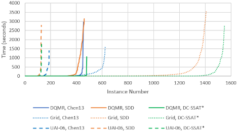
The results are shown in Table 2, where the format is similar to that of Table 1 and "#H" indicates the number of unobserved variables in the SDP queries. For the DQMR networks, DC-SSAT† and SDD solved all instances, while Chen13 only solved around two thirds of the instances. For the Grid benchmarks, DC-SSAT† and SDD outperformed Chen13*, and DC-SSAT† solved much more instances than SDD. For the UAI-06 benchmarks, DC-SSAT† and SDD solved fewer cases than Chen13*. Particularly, Chen13* uniquely solved several instances while DC-SSAT† and SDD tended to solve a similar set of instances.
6 The source code was given by the authors of [Chen et al., 2013].
7 https://github.com/wannesm/PySDD
| #Inst | #D | #L | limid | limid* | DC-SSAT | ClauSSat | |
|---|---|---|---|---|---|---|---|
| 120 | 3 | 3 | 47 / 0 | 120 / 0 | 120 / 0 | 120 / 0 | |
| DQMR | 120 | 5 | 3 | 35 / 0 | 120 / 0 | 120 / 0 | 120 / 0 |
| 120 | 8 | 3 | 33 / 0 | 120 / 0 | 120 / 0 | 120 / 0 | |
| Total | 360 | 115 / 0 | 360 / 0 | 360 / 0 | 360 / 0 | ||
| Grid | 450 | 3 | 7 | 117 / 1 | 262 / 0 | 393 / 19 | 219 / 0 |
| 450 | 5 | 11 | 87 / 0 | 240 / 0 | 364 / 15 | 216 / 0 | |
| 450 | 8 | 13 | 39 / 1 | 206 / 2 | 305 / 6 | 181 / 0 | |
| Total | 1350 | 243 / 2 | 708 / 2 | 1062 / 40 | 616 / 0 | ||
| UAI06 | 78 | 3 | 7 | 24 / 16 | 65 / 8 | 35 / 2 | 37 / 0 |
| 78 | 5 | 11 | 19 / 12 | 60 / 5 | 32 / 2 | 37 / 0 | |
| 78 | 8 | 10 | 15 / 8 | 59 / 8 | 33 / 2 | 37 / 1 | |
| Total | 234 | 58 / 36 | 184 / 21 | 100 / 6 | 111 / 0 |
The plot of Figure 4 compares the performance of the three solvers on the three benchmark sets separately. The x-axis corresponds to the number of solved instances with respect to a threshold runtime allowed to solve an instance in the yaxis. The result indicates that DC-SSAT† outperformed the other solvers in runtime for the DQMR and Grid benchmarks. For the UAI-06 benchmarks, Chen13* ran more efficiently than the other solvers, while DC-SSAT† and SDD had similar performance.
6.3 MEUComputation
For MEU computation, in each Bayesian network 3, 5, 10 of their chance nodes were selected randomly and replaced with decision nodes. In addition, two utility nodes each with three incoming edges were added in each benchmark instance. The influence diagram solver limid 8 , which implements the exact algorithm [Dechter, 2000] for the MEU problem, and the SSAT-based method using DC-SSAT and ClauSSat were studied. Also, we enhanced limid with the PGM preprocessing, denoted limid*, for study.
The results are shown in Table 3, where the format is similar to that of Table 1, "#D" indicates the number of decision nodes, and "#L" lists the maximum quantification level among a group of SSAT formulas. 9 For the DQMR benchmarks, both SSAT solvers solved all of them and outperformed limid. By the applied preprocessing, limid* can solve all the cases. For the Grid benchmarks, DC-SSAT solved the most instances and outperformed the other solvers. For the UAI-06 benchmarks, limid* completed more instances than SSAT solvers and uniquely solved several instances. The results suggested SSAT solvers can complement limid* in solving different instances.
7 RelatedWork
In [Sang et al., 2005], the conditional probabilities of a Bayesian network are encoded into a propositional formula for weighted model counting to answer the probability of evidence (PE) queries. In [Chavira and Darwiche, 2008], different types of encoding were discussed and the method ENC4 can greatly reduce the CNF formula size. We consider the binary encoding by using the indicator variables [Bart et al., 2016], which allows formula simplification with a two-level logic minimization tool. Because the PE problem is of #Pcomplete complexity, it is effectively an SSAT instance involving only one level of randomized quantification 10 and simply solvable by weighted model counting. In contrast, in the SSAT context of this work, the quantification prefix of a formula has to be explicitly considered.
8 https://github.com/radum2275/limid
9 We remark that the number of quantification levels is generally proportional to the number of decision nodes. However, because some decision nodes could be pruned by the reduction of Section 5.1, a instance with more decision nodes can possibly have fewer quantification levels in its SSAT encoding than another with fewer decision nodes. This phenomenon can be seen in the UAI-06 benchmarks, comparing #L=10 for #D=8 to #L=11 for #D=5.
Algorithms exploiting approximate solutions were developed, e.g., [Lee et al., 2021] for approximate MEU computation and [Marinescu et al., 2018] for approximate MAP computation. In contrast, this work focuses on exact computations and queries involving multiple quantifier alternations.
In [Majercik and Littman, 2003], the authors propose an SSAT encoding of the probabilistic propositional contingent planning problem represented in the sequential-effects-tree [Littman, 1997]. They exploit the prefix structure of SSAT to encode the causality relation that some information should be known before making a decision. They focus on the special case that the known information is one of two possible values, and have to modify the SSAT solver to be able to sum up the probabilities of two branches of some variable in SSAT solving. In contrast, in our case, the information known before making a decision can be one of arbitrary multiple states. Also, we do not modify the SSAT solver but recalculate the target solution using a scaling factor as is done in Eq. (20).
8 Conclusions
We have presented an SSAT-based approach to statistical inference, including MAP, SDP, and MEU queries on PGMs. It allows encoding of complex queries in PSPACE complexity class into SSAT formulas, in contrast to prior efforts on #Pcomplete and PP-complete problems. To test the feasibility of our methods, we have performed evaluation on MAP and SDP computations on Bayesian networks and MEU computation on influence diagrams. Experimental results suggested that our method can complement the state-of-the-art PGM tools in solving complex queries. For future work, we plan to relax our solution exactness to approximation to further extend the scalability.
Acknowledgments
This work was supported in part by the Ministry of Science and Technology of Taiwan under grants MOST 108-2221-E002-144-MY3 and MOST 109-2224-E-002-008.
@inproceedings{ijcai2022p255,
  title     = {Encoding Probabilistic Graphical Models into Stochastic Boolean Satisfiability},
  author    = {Hsieh, Cheng-Han and Jiang, Jie-Hong R.},
  booktitle = {Proceedings of the Thirty-First International Joint Conference on
               Artificial Intelligence, {IJCAI-22}},
  publisher = {International Joint Conferences on Artificial Intelligence Organization},
  editor    = {Luc De Raedt},
  pages     = {1834--1842},
  year      = {2022},
  month     = {7},
  note      = {Main Track},
  doi       = {10.24963/ijcai.2022/255},
  url       = {https://doi.org/10.24963/ijcai.2022/255},
}
TY - CPAPER TI - Encoding Probabilistic Graphical Models into Stochastic Boolean Satisfiability AU - Hsieh, Cheng-Han AU - Jiang, Jie-Hong R. T2 - Proceedings of the Thirty-First International Joint Conference on Artificial Intelligence, IJCAI-22 PB - International Joint Conferences on Artificial Intelligence Organization PY - 2022 SP - 1834 EP - 1842 DO - 10.24963/ijcai.2022/255 UR - https://doi.org/10.24963/ijcai.2022/255 ER -Copied
Machine-readable versions of this paper, for tools and AI agents:





