
Doubly Sparse Asynchronous Learning for Stochastic Composite Optimization
Proceedings of the Thirty-First International Joint Conference on Artificial Intelligence. Main Track. Pages 1916-1922.
https://doi.org/10.24963/ijcai.2022/266
Keywords
- Data Mining: Parallel, Distributed and Cloud-based High Performance Mining
- Machine Learning: Optimisation
- Data Mining: Big Data and Scalability
- Machine Learning: Feature Extraction, Selection and Dimensionality Reduction
Abstract
Parallel optimization has become popular for large-scale learning in the past decades. However, existing methods suffer from huge computational costs, memory usage, and communication burden in high-dimensional scenarios. To address the challenges, we propose a new accelerated doubly sparse asynchronous learning (DSAL) method for stochastic composite optimization, under which two algorithms are proposed on shared-memory and distributed-memory architecture respectively, which only conducts gradient descent on the nonzero coordinates (data sparsity) and active set (model sparsity). The proposed algorithm can converge much faster and achieve significant speedup by simultaneously enjoying the sparsity of the model and data. Moreover, by sending the gradients on the active set only, communication costs are dramatically reduced. Theoretically, we prove that the proposed method achieves the linear convergence rate with lower overall complexity and can achieve the model identification in a finite number of iterations almost surely. Finally, extensive experimental results on benchmark datasets confirm the superiority of our proposed method.
- [Agarwal and Duchi, 2012] Alekh Agarwal and John C Duchi. Distributed delayed stochastic optimization. In IEEE CDC, 2012.
- [Bao et al., 2019] Runxue Bao, Bin Gu, and Heng Huang. Efficient approximate solution path algorithm for ordered weighted l 1-norm with accuracy guarantee. In IEEE ICDM, 2019.
- [Bao et al., 2020] Runxue Bao, Bin Gu, and Heng Huang. Fast oscar and owl with safe screening rules. In ICML, 2020.
- [Bogdan et al., 2015] Małgorzata Bogdan, Ewout Van Den Berg, Chiara Sabatti, et al. Slope-adaptive variable selection via convex optimization. Ann. Appl. Stat, 2015.
- [Chang and Lin, 2011] Chih-Chung Chang and Chih-Jen Lin. Libsvm: A library for support vector machines. ACM TIST, 2011.
- [Dean et al., 2012] Jeffrey Dean, Greg Corrado, Rajat Monga, et al. Large scale distributed deep networks. In NeurIPS, 2012.
- [Ghaoui et al., 2010] Laurent El Ghaoui, Vivian Viallon, and Tarek Rabbani. Safe feature elimination in sparse super- vised learning. Technical report, 2010.
- [Gui and Li, 2005] Jiang Gui and Hongzhe Li. Penalized cox regression analysis in the high-dimensional and low- sample size settings, with applications to microarray gene expression data. Bioinformatics, 2005.
- [Joulani et al., 2019] Pooria Joulani, András György, and Csaba Szepesvari. Think out of the "box": Generically- constrained asynchronous composite optimization and hedging. NeurIPS, 2019.
- [Langford et al., 2009] John Langford, Alexander J Smola, and Martin Zinkevich. Slow learners are fast. In NeurIPS, 2009.
- [Leblond et al., 2017] Rémi Leblond, Fabian Pedregosa, and Simon Lacoste-Julien. Asaga: asynchronous parallel saga. In AISTATS, 2017.
- [Leblond et al., 2018] Rémi Leblond, Fabian Pedregosa, and Simon Lacoste-Julien. Improved asynchronous parallel optimization analysis for stochastic incremental methods. JMLR, 2018.
- [Li et al., 2016a] Qingyang Li, Shuang Qiu, Shuiwang Ji, et al. Parallel lasso screening for big data optimization. In ACM SIGKDD, 2016.
- [Li et al., 2016b] Yitan Li, Linli Xu, Xiaowei Zhong, and Qing Ling. Make workers work harder: decoupled asyn- chronous proximal stochastic gradient descent. arXiv preprint arXiv:1605.06619, 2016.
- [Lian et al., 2015] Xiangru Lian, Yijun Huang, Yuncheng Li, and Ji Liu. Asynchronous parallel stochastic gradient for nonconvex optimization. In NeurIPS, 2015.
- [Meng et al., 2017] Qi Meng, Wei Chen, Jingcheng Yu, et al. Asynchronous stochastic proximal optimization al- gorithms with variance reduction. In AAAI, 2017.
- [Ndiaye et al., 2017] Eugene Ndiaye, Olivier Fercoq, Alexandre Gramfort, et al. Gap safe screening rules for sparsity enforcing penalties. JMLR, 2017.
- [Ng, 2004] Andrew Y Ng. Feature selection, l 1 vs. l 2 regu- larization, and rotational invariance. In ICML, 2004.
- [Nguyen et al., 2018] Lam Nguyen, Phuong Ha Nguyen, Marten Dijk, et al. Sgd and hogwild! convergence without the bounded gradients assumption. In ICML, 2018.
- [Pedregosa et al., 2017] Fabian Pedregosa, Rémi Leblond, and Simon Lacoste-Julien. Breaking the nonsmooth bar- rier: A scalable parallel method for composite optimiza- tion. In NeurIPS, 2017.
- [Recht et al., 2011] Benjamin Recht, Christopher Ré, Stephen J Wright, et al. Hogwild: A lock-free approach to parallelizing stochastic gradient descent. In NeurIPS, 2011.
- [Reddi et al., 2015] Sashank J Reddi, Ahmed Hefny, Suvrit Sra, et al. On variance reduction in stochastic gradient descent and its asynchronous variants. In NeurIPS, 2015.
- [Stich et al., 2021] Sebastian Stich, Amirkeivan Mo- htashami, and Martin Jaggi. Critical parameters for scalable distributed learning with large batches and asynchronous updates. In AISTATS, 2021.
- [Tibshirani and others, 2013] Ryan J Tibshirani et al. The lasso problem and uniqueness. Electron. J. Stat., 2013.
- [Tibshirani et al., 2012] Robert Tibshirani, Jacob Bien, Jerome Friedman, et al. Strong rules for discarding predictors in lasso-type problems. JRSS, 2012.
- [Tibshirani, 1996] Robert Tibshirani. Regression shrinkage and selection via the lasso. JRSS, 1996.
- [Wang et al., 2012] Gang Wang, Derek Hoiem, and David Forsyth. Learning image similarity from flickr groups us- ing fast kernel machines. IEEE TPAMI, 2012.
- [Wu et al., 2013] Xindong Wu, Xingquan Zhu, Gong-Qing Wu, and Wei Ding. Data mining with big data. IEEE TKDE, 2013.
- [Xiao and Zhang, 2014] Lin Xiao and Tong Zhang. A prox- imal stochastic gradient method with progressive variance reduction. SIOPT, 2014.
- [Yuan and Lin, 2006] Ming Yuan and Yi Lin. Model selec- tion and estimation in regression with grouped variables. JRSS, 2006.
- [Zhang and Kwok, 2014] Ruiliang Zhang and James Kwok. Asynchronous distributed admm for consensus optimiza- tion. In ICML, 2014.
- [Zhang et al., 2016] Ruiliang Zhang, Shuai Zheng, and James T Kwok. Asynchronous distributed semi-stochastic gradient optimization. In AAAI, 2016.
- [Zhao and Li, 2016] Shen-Yi Zhao and Wu-Jun Li. Fast asynchronous parallel stochastic gradient descent: A lock- free approach with convergence guarantee. In AAAI, 2016.
- [Zhou et al., 2018] Kaiwen Zhou, Fanhua Shang, and James Cheng. A simple stochastic variance reduced algorithm with fast convergence rates. In ICML, 2018.
References were extracted automatically from the PDF and may contain errors.
Full text extracted automatically from the PDF; figures, tables and equations may differ. The PDF is the version of record.
1 Introduction
Big data with massive samples and numerous features recently widely exists in many real-world machine learning tasks, which often contains superfluous features [Gui and Li, 2005]. In the past decades, many models with sparse regularization have achieved great successes in high-dimensional scenarios by encouraging the model sparsity [Tibshirani, 1996; Ng, 2004; Yuan and Lin, 2006; Bao et al., 2019]. Let A = [a1, · · · , an]⊤ ∈ ℜn×p , in this paper, we consider the following composite optimization problem:
where x is the model coefficient, Ω(x) is the block-separable sparsity-inducing norm, F(x) = 1n ∑ni=1 fi(a⊤i x) is the data-fitting loss, and λ is the regularization parameter. We denote Fi(x) = fi(a⊤i x) for simplicity. Given partition G of the coefficients, we denote the sub-matrix of A with the columns of Gj as Aj ∈ ℜn×|Gj | and have Ω(x) = ∑qj=1 Ωj(xGj ).
∗This work was partially supported by NSF IIS 1845666, 1852606, 1838627, 1837956, 1956002, 2040588.
Inspired by the emerging parallel computing systems such as multi-core computer and distributed architecture, parallel learning has been actively studied in machine learning community due to its capability for tackling large-scale applications [Wang et al., 2012; Wu et al., 2013]. In literature, many parallel learning methods have been proposed to accelerate different optimization algorithms on shared-memory architecture [Langford et al., 2009; Recht et al., 2011; Reddi et al., 2015; Zhao and Li, 2016; Leblond et al., 2017; Meng et al., 2017; Pedregosa et al., 2017; Zhou et al., 2018; Leblond et al., 2018; Nguyen et al., 2018; Joulani et al., 2019; Stich et al., 2021] and distributed-memory architecture [Agarwal and Duchi, 2012; Dean et al., 2012; Zhang and Kwok, 2014; Lian et al., 2015; Zhang et al., 2016]. For smooth optimization problems, asynchronous stochastic methods, e.g., Hogwild! [Recht et al., 2011], Lock-Free SVRG [Reddi et al., 2015], AsySVRG [Zhao and Li, 2016], and ASAGA [Leblond et al., 2017], were proposed. Furthermore, AsyProxSVRG [Meng et al., 2017], ProxASAGA [Pedregosa et al., 2017], and AsyMiG [Zhou et al., 2018] were proposed to solve non-smooth composite optimization problems. However, most existing methods focus on improving the algorithm efficiency in terms of sample complexity.
To solve the problems with huge samples and features, an asynchronous doubly stochastic method was proposed in [Meng et al., 2017], which performs coordinate updates without considering any sparsity and thus can be very slow. Moreover, [Leblond et al., 2017] proposed an asynchronous sparse incremental gradient method, which does not enjoy the sparsity of the model to accelerate the training and thus huge requirement of computational complexity hinders its application on large-scale learning. Therefore, existing parallel methods still suffer huge burden for computation, memory, and communication costs to solve high-dimensional models.
In high-dimensional setting, sparsity is a key property that can be exploited to accelerate the training. Sparsity can be broken down into two aspects: data sparsity and model sparsity. In terms of the data sparsity, the dataset usually has a huge number of features in which most of the elements are zero. If the feature representation of the current sample is zero, the stochastic gradient w.r.t. the corresponding feature must be zero. It is an effective method to accelerate the training by avoiding the useless updates of these gradients. On the other aspect, the regularization usually enforces the model sparsity where the coefficients of the associated features are zeroes at the optimum. The model sparsity can be exploited to reduce the problem dimensionality by pre-identifying inactive features [Ndiaye et al., 2017; Bao et al., 2020]. Discarding these features can save much computation without any loss of accuracy. Therefore, accelerating high-dimensional models by exploiting the sparsity is promising and sorely needed for large-scale problems.
| Reference | Model | Dynamic | Safe | Distributed | Scalablity | Data Sparsity |
|---|---|---|---|---|---|---|
| PE-AGCD [Li et al., 2016a] | Lasso | No | No | No | No | No |
| DSAL (Ours) | Problem (1) | Yes | Yes | Yes | Yes | Yes |
To address the challenges above, in this paper, we propose a novel accelerated doubly sparse asynchronous learning (DSAL) method for stochastic composite optimization and apply it on shared-memory (Sha-DSAL) and distributedmemory (Dis-DSAL) architecture, which can accelerate the training significantly without any loss of accuracy. Specifically, DSAL not only conducts the elimination to discard inactive features to enjoy the model sparsity, but also conducts sparse proximal gradient update with the nonzero partial gradients to enjoy the data sparsity. To further accelerate DSAL, we reduce the gradient variance over the active set and thus can utilize a constant step size to achieve the linear convergence. On distributed-memory system, to reduce the computational burden of the server, we utilize a decouple strategy to improve the scalability of DSAL w.r.t. the number of workers.
Contributions. The main contributions of our work are summarized as follows:
- We propose a new doubly sparse asynchronous stochastic gradient method for stochastic composite optimization, which is easy-to-implement on the both sharedmemory and distributed-memory architecture. To the best of our knowledge, this is the first work of asynchronous stochastic gradient method to simultaneously enjoy the model sparsity and data sparsity.
- We rigorously prove the DSAL method can achieve a linear convergence rate O(log(1/ϵ)), reduce the periteration cost from O(p) to O(r) where r ≪ p, and achieve a lower overall computational complexity under the strongly convex condition. Moreover, we prove almost sure finite time identification of the active set.
- We empirically show that our proposed method can simultaneously achieve significant acceleration and linear speedup property.
1.1 RelatedWorks
Parallel method (PE-AGCD) in [Li et al., 2016a] handles the high-dimensional setting by conducting the parallel elimination (PE) step before Asynchronous Grouped Coordinate Descent (AGCD). However, the proposed method has several disadvantages. First, PE is only conducted once prior to the optimization algorithm. Second, only safe static rule [Ghaoui et al., 2010] used in PE is safe and the strong rule [Tibshirani et al., 2012] used in PE is unsafe, which means it could discard features wrongly. Third, PE-AGCD is deterministic on samples and thus cannot scale well for large n. Fourth, PE-AGCD cannot enjoy the sparsity of the data. Lastly, PEAGCD is limited to Lasso regression. Table 1 summarizes the advantages of our DSAL over PE-AGCD. First, DSAL is dynamic and conducted during the whole training process. Thus, DSAL can accelerate and meanwhile benefit from the convergence of the optimization algorithm. Second, our DSAL is safe for the training. Third, DSAL is stochastic and can scale well on both samples and features. Fourth, DSAL can enjoy the data sparsity by performing sparse proximal updates. Lastly, DSAL can solve Problem (1).
2 ProposedMethod
We first propose the accelerated doubly sparse asynchronous learning (DSAL) method and then apply it to shared-memory and distributed-memory architecture respectively.
2.1 Doubly Sparse Asynchronous Learning
To enjoy the sparsity of the model coefficient, we first give a naive implementation of DSAL on shared-memory architecture in Alg. 1. During the training, DSAL only need solve a sub-problem with constantly decreasing size by discarding useless features. Specifically, Alg. 1 has two loops. We denote the original problem as P0 and the full set as B0. At the s-th iteration of the outer loop, we denote the active set as Bs and suppose Bs has qs active blocks with total ps active features. Then we can compute the dual ys as
where dual norm ΩD (u) = maxΩ(v)≤1⟨v, u⟩. Then, for ∀j ∈ Bs, Bs+1 is updated by:
where L is the Lipschitz constant and D(ys ) is the dual objective of Ps ([Ndiaye et al., 2017; Bao et al., 2020]).
For the inner loop, all the updates are conducted on Bs+1. First, each thread inconsistently reads ˆxtBs+1 from the shared memory and randomly chooses sample i to compute the stochastic gradient on Bs+1. Then, the proximal step is conducted with the stochastic gradient. By (3), we can constantly reduce the model size and the parameter size to accelerate the training by exploiting the sparsity of the model. Since each variable xi discarded by the elimination must be zero for the optimum solution, this method is safe for the training.
Algorithm 1 Sha-DSAL-Naive
1: Input: x0B0 ∈ ℜp , step size η, inner loops K. 2: for s = 0 to S -1 do 3: All threads parallelly compute ∇F(x0Bs ) 4: Compute ys by (2) and Bs+1 fromBs by (3) 5: Update ABs+1 , x0Bs+1 6: For each thread, do: 7: for t = 0 to K - 1 do 8: Read ˆxtBs+1 from the shared memory 9: Randomly sample i from {1, 2, . . . , n} 10: vs t =∇fi(a⊤i,Bs+1 ˆxtBs+1 ) 11: Update xt+1 Bs+1 = proxηλΩ(ˆxtBs+1 - ηvs t ) 12: end for 13: xBs+1 = xKBs+1 , x0Bs+1 = xBs+1- 14: end for
Variance Reduction on the Active Set
However, the variance of the gradient in Alg. 1 caused by stochastic sampling does not converge to zero. Thus, we have to use a diminishing step size and can only attain a sublinear convergence rate when P is strongly convex.
Since the full gradient has been computed for the elimination step, inspired by [Xiao and Zhang, 2014], we can adopt the variance-reduced technique over active set Bs+1 without additional computational costs. Thus, we can adjust the gradient estimation as
which can guarantee that the variance of stochastic gradients asymptotically converges to zero. Therefore, we can use a constant step size to achieve a linear convergence rate for strongly convex function.
Sparse Proximal Gradient Update
In practice, sparsity widely exists in large-scale datasets. To utilize the data sparsity, we only need to update the blocks with nonzero partial gradients. Thus, some blocks might be updated for more times while others for less times. Inspired by [Leblond et al., 2017] for Proximal SAGA, we define a block-wise reweighting matrix to make a weighted projection on the blocks. Specifically, we define Ψi as the set of blocks that intersect the nonzero coefficients of ∇fi. Let nG be the number of occurrences that G ∈ Ψi, if nG > 0, we define dG = n/nG. Otherwise, we ignore that block directly. Thus, we can define diagonal matrix [Di]G,G = dGI|G| for each block i and the gradient over Bs+1 can be formulated as
Thus, we only need conduct a sparse update over the active set and the computational cost is further reduced.
On the other hand, the proximal operator of Problem (1) needs to update all the coordinates for each iteration. Considering the data sparsity again, we only need to update the blocks with nonzero partial gradients. Thus, we use a blockwise weighted norm ϕi(x) = ∑G∈Ψi dGΩG(x) to displace Ω(x) where Eϕi(x) = Ω(x). Thus, the new sparse proximal operator can be computed as
Since we only need to update the blocks in Ψi, which could be much less than the full pass, we can save much computation and memory cost here. To sum it up, we can conduct the sparse gradient update and sparse proximal operator to accelerate the training by enjoying the sparsity of the data.
Decoupled Proximal Update
On distributed-memory architecture, multiple workers compute the gradients and send them to the server. The server computes the proximal operator. When the proximal step is time-consuming, doing this in the server would be the computational bottleneck of the whole algorithm. [Li et al., 2016b] proposed a decoupled method to off-load the computations of the proximal step to workers. Thus, the server only does simple addition computation, which can achieve a sublinear converge rate and perform better than the coupled method.
To relieve the computation cost of the server in our algorithm, the proximal mapping step is computed by workers and the server only needs to do the element-wise computation. The workers conduct the proximal operator as xt+1 Bs+1 = proxηλϕi (xtBs+1 - ηvs t ) and send the difference δs t = proxηλϕi (xd(t) Bs+1 - ηvs t ) - xd(t) Bs+1 between the parameter xd(t) Bs+1 and the output of the proximal operator to the server. Therefore, the server only does simple addition computation, which makes the algorithm suitable to parallelize to achieve linear speedup property and can be accelerated via increasing the number of workers.
2.2 DSAL on Shared-Memory and Distributed-Memory Architecture
On shared-memory architecture, our Sha-DSAL algorithm is in Alg. 2. Suppose we have l cores, in the outer loop, all threads parallelly compute ∇F(x0Bs ) and ys , and perform the elimination. With new set Bs+1, we update ABs+1 , x0Bs+1 , and ∇F(x0Bs+1 ). In the inner loop, multiple threads update the parameter over Bs+1 asynchronously, which means the parameter can be read and written without locks. Specifically, each thread inconsistently read ˆxtBs+1 from the shared memory and choose sample i. As (5), we compute the gradient vs t over Bs+1. Then we conduct the proximal step, compute the update δs t , and add it to the shared memory.
Notably, first, at the s-th iteration, by exploiting the sparsity of the model, our Alg. 2 only solve sub-problem Ps+1 over Bs+1, which is much more efficient than training the full model. The full gradients at the s-th iteration in our algorithm is only computed with ps coefficients, which is much less than O(p) in practice. Second, by exploiting the data sparsity, we only conduct sparse gradient update and sparse proximal update, which is very efficient for large-scale dataset. Third, by reducing the gradient variance, we can use a constant step size to achieve a linear convergence rate. Lastly, all
Algorithm 2 Sha-DSAL
- 1: Input: x0B0 ∈ ℜp , step size η, inner loops K. 2: for s = 0 to S -1 do 3: All threads parallelly compute ∇F(x0Bs ) 4: Compute ys by (2) and Bs+1 fromBs by (3) 5: Update ABs+1 , x0Bs+1 ,∇F(x0Bs+1 ) 6: For each thread, do: 7: for t = 0 to K - 1 do 8: Read ˆxtBs+1 from the shared memory 9: Randomly sample i from {1, 2, . . . , n} 10: Compute vs t by (5) 11: δs t = proxηλϕi (ˆxtBs+1 - ηvs t ) - ˆxtBs+1 12: xt+1 Bs+1 = xtBs+1 + δs t 13: end for 14: xBs+1 = xKBs+1 , x0Bs+1 = xBs+1 15: end for
the threads work asynchronously, which is very easy to parallelize. Hence, the computation, memory, and communication costs of large-scale training can be effectively reduced.
On distributed-memory architecture, our Dis-DSAL algorithm is summarized in Alg. 3 and 4. Suppose we have one server node and l local worker nodes where each worker stores nk samples. When the flag is True, in the outer loop of the server, the server broadcasts the flag and x0Bs to the workers. At the worker node, worker k receives x0Bs from the server, computes the gradient over nk samples, and then sends them to the server. With the gradients received from all the workers, the server computes the full gradients and send them to the workers. Then, the server computes ys , performs the elimination to obtain Bs+1, and then send it to the workers. The worker receives ∇F(x0Bs ) and Bs+1 from the server. With Bs+1, the worker updates Ai∈nk,Bs+1 , x0Bs+1 and ∇F(x0Bs+1 ). When the flag is False, the server broadcasts the flag to the workers. At the workers, the algorithm optimizes over Bs+1. Multiple workers update the parameter asynchronously. Specifically, each worker receives stale parameter xd(t) Bs+1 from the server. The worker first chooses sample i from {1, 2, . . . , nk} and compute vs t over Bs+1. Following the decoupling strategy, we compute the proximal step and the update at the worker node. Finally, the worker send it to server. In the inner loop of the server, xt+1 Bs+1 is updated by δs t fromworkers via only simple addition computation.
Similar to Alg. 2, our Alg. 3 and 4 is computationally efficient by exploiting the sparsity of the model and the dataset and reducing the gradient variance. Moreover, the time-consuming proximal step from the server is off-loaded to all the workers, which is easy to parallelize. Overall, the computation, memory, and communication costs could be effectively reduced.
3 Theoretical Analysis
We provide the rigorous theoretical analysis for DSAL on shared-memory architecture, which can be easily extended to distributed memory. The proof is provided in the appendix.
Algorithm 3 Dis-DSAL (Server Node)
- 1: for s = 0 to S -1 do
- 2: flag = True
- 3: Broadcast flag and x0Bs to all workers
- 4: Receive gradients from all workers
- 5: ∇F(x0Bs ) = 1n ∑lk=1 ∇Fk(x0Bs )
- 6: Compute ys by (2) and update Bs+1 ⊆ Bs by (3)
- 7: Broadcast Bs+1 and ∇F(x0Bs ) to all workers
- 8: flag = False
- 9: Broadcast flag to all workers
- 10: for t = 0 to K - 1 do
- 11: Receive δs t from one worker
- 12: Update xt+1 Bs+1 = xtBs+1 + δs t
- 13: end for
- 14: xBs+1 = xKBs+1 , x0Bs+1 = xBs+1
- 15: end for
Algorithm 4 Dis-DSAL (Worker Node k)
- 1: if flag = True then
- 2: Receive x0Bs from server
- 3: Compute and send gradient ∇Fk(x0Bs ) = ∑i∈nk ∇fi(a⊤i,Bs x0Bs )
- 4: Receive ∇F(x0Bs ) and Bs+1 from server
- 5: Update Ai∈nk,Bs+1 , x0Bs+1 ,∇F(x0Bs+1 )
- 6: else
- 7: Receive xd(t) Bs+1 from server
- 8: Randomly sample i from {1, 2, . . . , nk}
- 9: Compute vs t = ∇fi(a⊤i,Bs+1 xd(t) Bs+1 ) - ∇fi(a⊤i,Bs+1 x0Bs+1 ) + Di,Bs+1 ∇F (x0Bs+1 )
- 10: Send δt = proxηλϕi (xd(t) Bs+1 - ηvs t ) - xd(t) Bs+1 to server
- 11: end if
3.1 Assumptions, Definitions, and Properties
Assumption 1 (Strong Convexity). Ω(x) is convex and block separable. F(x) is µ-strongly convex, i.e., ∀x, x′ ∈ ℜp , we have F(x′ ) ≥ F(x) + ∇F(x)⊤(x′ - x) + µ2 ∥x′ - x∥2 .
Assumption 2 (Lipschitz Smooth). Each Fi(x) is differentiable and Lipschitz gradient continuous with L, i.e., ∃L > 0, such that ∀x, x′ ∈ ℜp , we have ∥∇Fi(x) -∇Fi(x′ )∥ ≤ L∥x - x′ ∥.
Assumption 3 (Bounded Overlapping). There exists a bound τ on the number of iterations that overlap. The bound τ means each writing at iteration t is guaranteed to successfully performed into the memory before iteration t + τ + 1.
Remark 1. Asm. 1 implies P(x) is also µ-strongly convex. Asm. 2 implies that F(x) is also Lipschitz gradient continuous. We denote κ := L/µ as the condition number. Asm. 3 means the delay that asynchrony may cause is upper bounded. All the assumptions are commonly seen in asynchronous methods [Pedregosa et al., 2017].
Definition 1 (Block Sparsity). We denote that the maximum frequency of occurrences ∆ that a feature block belongs to the extended support, which can be defined as ∆ = maxG∈B |{i : Ψi ∋ G}|/n. It is easy to verify that 1/n ≤ ∆ ≤ 1.
Property 1 (Independence). We use the "after read" labeling in [Leblond et al., 2017], which means we update the iterate counter after each thread fully reads the parameters. This means that ˆxtBs+1 is the (t+1)-th fully completed read. Given the "after read" global time counter, sample ir is independent of ˆxtBs+1 , ∀r ≥ t.
Property 2 (Unbiased Gradient Estimation). Gradient vt is an unbiased estimation of the gradient over set Bs+1 at ˆxtBs+1 , which is directly derived from Property 1.
Property 3 (Atomic Operation). The update xt+1 Bs+1 to shared memory in Alg. 2 is coordinate-wise atomic, which can address the overwriting problem caused by other threads.
3.2 Theoretical Results
Theorem 1 (Convergence). Suppose τ ≤ 1 10√∆ , let step size η = min{ 1 24κL , κ 2L , κ 10τL }, inner loop size K = 4 log 3 ηµ , we have
Remark 2. Theorem 1 shows that DSAL can achieve a linear convergence rate O(log(1/ϵ)).
Remark 3. For the case F(x) is nonstrongly convex, we can slightly modify Ω(x) by adding a small perturbation, e.g., µf∥x∥2 for smoothing where µf > 0. We can treat F(x) + µf∥x∥2 as the data-fitting loss and then the loss is µf -strongly convex. Denote κ := L/µf , suppose τ ≤ 1 10√∆ , let η = min{ 1 24κL , κ 2L , κ 10τL }, K = 4 log 3 ηµf , we have E ∥∥xBS - x∗BS ∥∥2 ≤ (2/3)S ∥x0 - x∗ ∥2 .
Theorem 2 (Elimination Ability). Equicorrelation set [Tibshirani and others, 2013] is defined as B∗ := {j ∈ {1, 2, . . . , q} : ΩDj (A⊤j y∗ ) = nλ}. As DSAL converges, there exists an iteration number S0 ∈ N, s.t. ∀s ≥ S0, any variable block j /∈ B∗ is eliminated by DSAL almost surely.
Remark 4. Suppose the size of set Bs is ps and p∗ is the size of the active features in B∗ , Theorem 2 shows we have ps is decreasing and lims→+∞ ps = p∗ .
Remark 5. To sum it up, by the elimination, the cost at each iteration is reduced from O(p) to O(ps). Moreover, by the sparse update, only the nonzero coefficients of set Bs is updated and thus the cost at each iteration is further reduced from O(ps) to O(p′s ) where p′s is the size of the nonzero coefficients. In the high-dimensional setting, we have p∗ ≪ p, ps ≪ p and p′s ≪ p. Thus, with constantly decreasing ps and the sparse update, our DSAL can reduced the complexity from O(p) to O(r) where r is the mean of p′s for s = 1, 2, . . ., which can accelerate the training at a large extent in practice.
4 Experiments
4.1 Experimental Setup
We compare our method with competitive methods on three large-scale datasets. Although DSAL can work broadly, we focus on Lasso, which is the most popular case for sparse regression. Specifically, Lasso solves
On shared-memory architecture, we compare six asynchronous methods: 1) PE-Strong-AGCD: parallel strong elimination in [Li et al., 2016a]; 2) PE-Safe-AGCD: parallel static safe elimination in [Li et al., 2016a]; 3) ProxASAGA [Pedregosa et al., 2017]; 4) ProxASVRG [Meng et al., 2017]; 5) Sha-DSAL-Naive; 6) Our Sha-DSAL. ProxASAGA and ProxASVRG are popular asynchronous method with linear convergence. On distributed-memory architecture, we compare four asynchronous methods: 1) ProxASAGA [Leblond et al., 2018]; 2) ProxASVRG [Meng et al., 2017]; 3) DisDSAL-Naive (See appendix); 4) Our Dis-DSAL.
| Dataset | Sample Size | Attributes | Sparsity |
|---|---|---|---|
| KDD 2010 | 19,264,097 | 1,163,024 | 7×10⁻⁶ |
| Avazu-app | 14,596,137 | 1,000,000 | 10-5 |
| Avazu-site | 25,832,830 | 1,000,000 | 10-5 |
We use three real-world datasets in Table 2, which are from LIBSVM [Chang and Lin, 2011] at https://www.csie.ntu.edu. tw/∼cjlin/libsvmtools/datasets/. We implement all the methods in C++. We employ OpenMP and OpenMPI as the parallel framework for shared-memory and distributed-memory architecture respectively. We run all the methods on 2.10 GHz Intel(R) Xeon(R) CPU machines. The inner loop size and the step size are chosen to obtain the best performance. Parameter λ is selected as 4 ∗ 10-6λmax, 2 ∗ 10-3λmax, and 1 ∗ 10-3λmax for KDD 2010, Avazu-app, and Avazu-site dataset respectively where λmax is a parameter that, for all λ ≥ λmax, x∗ must be 0.
4.2 Experimental Results and Discussions
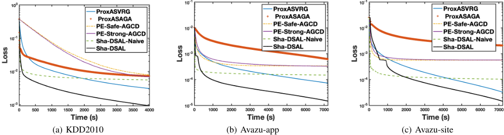
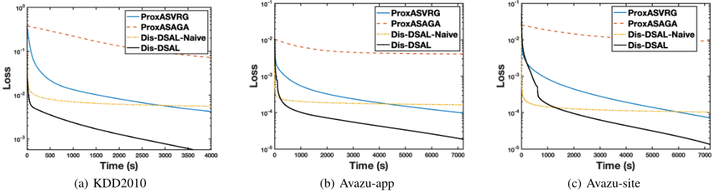
Convergence Results. Figure 1 (a)-(c) provides the convergence results on shared-memory architecture. Our ShaDSAL-Naive converges very fast at the initial stage because of the elimination ability and slows down later due to its sublinear rate. The results confirm that our Sha-DSAL always converge much faster than other methods. Figure 2 (a)-(c) provides the convergence results on distributed-memory architecture. The results also show that our Dis-DSAL always converge much faster than other methods. This is because our method can eliminate the features by exploiting the sparsity of the model, perform efficient sparse update by exploiting the data sparsity, achieve the linear convergence rate by reducing the gradient variance. Our Dis-DSAL also performs the decouple proximal update to reduce the workload of the server and reduces the communication costs.
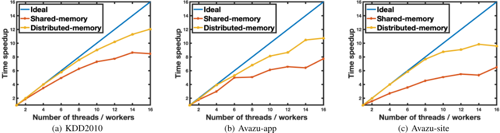
Linear Speedup Property. Figure 3(a)-(c) presents the results of the speedup of Sha-DSAL with different number of threads on shared-memory architecture and Dis-DSAL with different number of workers on distributed-memory architecture. The results show our method can successfully achieve a nearly linear speedup when we increase the number of threads or workers, although the performance decreases when the number of processors or works increases. This is because theoretical analysis does not take the overheads for creating threads and distributing work for OpenMP and communication costs for OpenMPI into account.
5 Conclusion
In this paper, we propose the first doubly sparse asynchronous learning method for stochastic composite optimization and apply it on shared-memory and distributed-memory architecture respectively. Theoretically, we prove that our proposed method can achieve a linear convergence rate with lower overall complexity. Moreover, our method can eliminate almost all the inactive variables in a finite number of iterations almost surely. Finally, numerical results confirm the superiority of our method. Since we only consider the blockseparable norm here, applying our method to non-separable norms, such as OWL regression [Bogdan et al., 2015; Bao et al., 2019], would be an interesting direction for future work.
@inproceedings{ijcai2022p266,
  title     = {Doubly Sparse Asynchronous Learning for Stochastic Composite Optimization},
  author    = {Bao, Runxue and Wu, Xidong and Xian, Wenhan and Huang, Heng},
  booktitle = {Proceedings of the Thirty-First International Joint Conference on
               Artificial Intelligence, {IJCAI-22}},
  publisher = {International Joint Conferences on Artificial Intelligence Organization},
  editor    = {Luc De Raedt},
  pages     = {1916--1922},
  year      = {2022},
  month     = {7},
  note      = {Main Track},
  doi       = {10.24963/ijcai.2022/266},
  url       = {https://doi.org/10.24963/ijcai.2022/266},
}
TY - CPAPER TI - Doubly Sparse Asynchronous Learning for Stochastic Composite Optimization AU - Bao, Runxue AU - Wu, Xidong AU - Xian, Wenhan AU - Huang, Heng T2 - Proceedings of the Thirty-First International Joint Conference on Artificial Intelligence, IJCAI-22 PB - International Joint Conferences on Artificial Intelligence Organization PY - 2022 SP - 1916 EP - 1922 DO - 10.24963/ijcai.2022/266 UR - https://doi.org/10.24963/ijcai.2022/266 ER -Copied
Machine-readable versions of this paper, for tools and AI agents:





