
CADET: Calibrated Anomaly Detection for Mitigating Hardness Bias
Proceedings of the Thirty-First International Joint Conference on Artificial Intelligence. Main Track. Pages 2002-2008.
https://doi.org/10.24963/ijcai.2022/278
Keywords
- AI Ethics, Trust, Fairness: Trustworthy AI
- Data Mining: Anomaly/Outlier Detection
Abstract
The detection of anomalous samples in large, high-dimensional datasets is a challenging task with numerous practical applications. Recently, state-of-the-art performance is achieved with deep learning methods: for example, using the reconstruction error from an autoencoder as anomaly scores. However, the scores are uncalibrated: that is, they follow an unknown distribution and lack a clear interpretation. Furthermore, the reconstruction error is highly influenced by the `hardness' of a given sample, which leads to false negative and false positive errors. In this paper, we empirically show the significance of this hardness bias present in a range of recent deep anomaly detection methods. To mitigate this, we propose an efficient and plug-and-play error calibration method which mitigates this hardness bias in the anomaly scoring without the need to retrain the model. We verify the effectiveness of our method on a range of image, time-series, and tabular datasets and against several baseline methods.
- [Aggarwal, 2015] Charu C Aggarwal. Outlier analysis. In Data mining, pages 237-263. Springer, 2015.
- [An, 2015] Jinwon An. Variational Autoencoder based Anomaly Detection using Reconstruction Probability. In SNU Data Mining Center 2015-2 Special Lecture on IE, 2015.
- [Bartels et al., 1995] Richard H Bartels, John C Beatty, and Brian A Barsky. An introduction to splines for use in com- puter graphics and geometric modeling. Morgan Kauf- mann, 1995.
- [Chen et al., 2018] Zhaomin Chen, Chai Kiat Yeo, Bu Sung Lee, and Chiew Tong Lau. Autoencoder-based network anomaly detection. In 2018 Wireless Telecommunications Symposium (WTS), pages 1-5, 2018.
- [Cortés-Ciriano and Bender, 2019] Isidro Cortés-Ciriano and Andreas Bender. Concepts and applications of conformal prediction in computational drug discovery. arXiv preprint arXiv:1908.03569, 2019.
- [Deng and Hooi, 2021] Ailin Deng and Bryan Hooi. Graph neural network-based anomaly detection in multivariate time series. In Proceedings of the AAAI Conference on Ar- tificial Intelligence, volume 35, pages 4027-4035, 2021.
- [Dinh et al., 2016] Laurent Dinh, Jascha Sohl-Dickstein, and Samy Bengio. Density estimation using real nvp. arXiv preprint arXiv:1605.08803, 2016.
- [Eklund et al., 2015] Martin Eklund, Ulf Norinder, Scott Boyer, and Lars Carlsson. The application of conformal prediction to the drug discovery process. Annals of Math- ematics and Artificial Intelligence, 74(1):117-132, 2015.
- [Goodge and Hooi, 2022] Adam Goodge and Bryan Hooi. Lunar: Unifying local outlier detection methods via graph neural networks. In Proceedings of the AAAI Conference on Artificial Intelligence, volume 36, 2022.
- [Goodge et al., 2020] Adam Goodge, Bryan Hooi, See- Kiong Ng, and Wee Siong Ng. Robustness of autoencoders for anomaly detection under adversarial impact. In IJCAI, pages 1244-1250, 2020. IJCAI
- [Guo et al., 2017] Chuan Guo, Geoff Pleiss, Yu Sun, and Kilian Q Weinberger. On calibration of modern neural net- works. In International Conference on Machine Learning, pages 1321-1330. PMLR, 2017.
- [Lei et al., 2018] Jing Lei, Max G'Sell, Alessandro Rinaldo, Ryan J Tibshirani, and Larry Wasserman. Distribution-free predictive inference for regression. Journal of the Ameri- can Statistical Association, 113(523):1094-1111, 2018.
- [Menon and Williamson, 2018] Aditya Krishna Menon and Robert C Williamson. A loss framework for calibrated anomaly detection. In Proceedings of the 32nd Interna- tional Conference on Neural Information Processing Sys- tems, pages 1494-1504, 2018.
- [Naeini et al., 2015] Mahdi Pakdaman Naeini, Gregory Cooper, and Milos Hauskrecht. Obtaining well calibrated probabilities using bayesian binning. In Proceedings of the AAAI Conference on Artificial Intelligence, volume 29, 2015.
- [Pang et al., 2021] Guansong Pang, Chunhua Shen, Long- bing Cao, and Anton Van Den Hengel. Deep learning for anomaly detection: A review. ACM Computing Surveys (CSUR), 54(2):1-38, 2021.
- [Romano et al., 2019] Yaniv Romano, Evan Patterson, and Emmanuel J Candès. Conformalized quantile regression. arXiv preprint arXiv:1905.03222, 2019.
- [Romano et al., 2020] Yaniv Romano, Matteo Sesia, and Emmanuel J Candès. Classification with valid and adap- tive coverage. arXiv preprint arXiv:2006.02544, 2020.
- [Vovk et al., 2005] Vladimir Vovk, Alex Gammerman, and Glenn Shafer. Algorithmic learning in a random world. Springer Science & Business Media, 2005.
- [Vovk et al., 2020] Vladimir Vovk, Ivan Petej, Paolo Toc- caceli, Alexander Gammerman, Ernst Ahlberg, and Lars Carlsson. Conformal calibrators. In Conformal and Probabilistic Prediction and Applications, pages 84-99. PMLR, 2020.
- [Xiao et al., 2017] Han Xiao, Kashif Rasul, and Roland Vollgraf. Fashion-mnist: a novel image dataset for bench- marking machine learning algorithms. arXiv preprint arXiv:1708.07747, 2017.
- [Yao et al., 2019] Rong Yao, Chongdang Liu, Linxuan Zhang, and Peng Peng. Unsupervised anomaly detection using variational auto-encoder based feature extraction. In 2019 IEEE International Conference on Prognostics and Health Management (ICPHM), pages 1-7. IEEE, 2019.
- [Yu et al., 2011] Dong Yu, Jinyu Li, and Li Deng. Calibra- tion of confidence measures in speech recognition. IEEE Transactions on Audio, Speech, and Language Processing, 19(8):2461-2473, 2011.
- [Zhao et al., 2017] Chunhui Zhao, Xueyuan Li, and Haifeng Zhu. Hyperspectral anomaly detection based on stacked denoising autoencoders. Journal of Applied Remote Sens- ing, 11(4):042605, 2017.
- [Zhou and Paffenroth, 2017] Chong Zhou and Randy C Paf- fenroth. Anomaly detection with robust deep autoen- coders. In Proceedings of the 23rd ACM SIGKDD in- ternational conference on knowledge discovery and data mining, pages 665-674, 2017.
References were extracted automatically from the PDF and may contain errors.
Full text extracted automatically from the PDF; figures, tables and equations may differ. The PDF is the version of record.
1 Introduction
The rapid growth in large-scale sensor data has led to the need to monitor and detect unusual samples, or anomalies, automatically. This is of vital importance in a wide variety of applications, ranging from medical, spatio-temporal, industrial, and many others. Recently, there has been a surge of interest in the use of deep learning methods to achieve more accurate anomaly detection in high-dimensional data such as images, time series, and sensor data. For each sample, the anomaly detection algorithm will output an anomaly score, where a higher score indicates a higher likelihood of the sample being anomalous. In most practical cases, the proportion of anomalous samples is extremely low relative to the normal samples and it can be very difficult to acquire accurately labelled anomalies. Therefore, unsupervised techniques which focus on learning the distribution of only the normal data are most practical. Autoencoders are a particularly popular algorithm within this approach [Aggarwal, 2015; Chen et al., 2018]; the network is trained with a training set of all normal samples and the reconstruction error is used to determine anomalies from the unseen data.
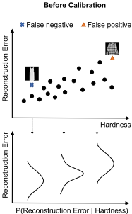
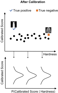
A major problem with many of these algorithms is that their anomaly scores are uncalibrated; that is, the scores follow an unknown distribution, and therefore lack a clear, consistent interpretation. In practice, flagging a sample as anomalous often results in manual inspection, which can be costly. Therefore, it is beneficial to have calibrated scores, which allow for a clear, consistent interpretation and measure how far a sample is away from the normal data distribution.
Calibration also helps to mitigate another significant problem for unsupervised anomaly detection methods, which we call the 'hardness bias'. We define 'hardness' formally in Section 3.2, but in short, hardness is an intrinsic and simple characteristic of a data sample to estimate how difficult it is to model a sample. Surprisingly, we find that existing anomaly detection approaches fail to take the effect of hardness into account, which leads to hardness bias and significant degradation in accuracy.
In this paper, we first show that a significant hardness bias exists in a range of deep anomaly detection methods through empirical observations with real data. We then propose our CADET framework for calibrated anomaly detection. Inspired by ideas from post-hoc calibration of machine learning models and the statistical framework of conformal prediction, this approach calibrates an anomaly detection algorithm to address the hardness bias problem while also providing (approximate) theoretical guarantees on false positive probability.
Overall, the benefits of our approach 1 are as follows:
- Generality: Our calibration framework can be flexibly applied on top of a wide variety of anomaly detection modules.
- Accuracy: By mitigating the problem of hardness bias, our approach consistently improves the accuracy of existing anomaly detection approaches.
- Efficiency: Our approach results in virtually no increase in overall computation time over the original anomaly detection approach (shown in the supplementary material) and requires no retraining of any pre-trained model.
- Probabilistic Guarantee: Unlike many existing approaches which return scores from an unknown distribution, our approach returns scores with a more clear and consistent interpretation, and provides a probabilistic guarantee decision rule that the false positive rate can be approximately tuned to a user-defined threshold ε > 0.
2 RelatedWork
2.1 Anomaly Detection
Unsupervised anomaly detection based on deep learning has led to a wide variety of approaches; see [Pang et al., 2021] for a survey. Typically, they learn a model of normal data, enabling them to identify anomalies which deviate from the learned distribution.
Reconstruction-based methods are one of the most popular anomaly detection approaches, especially for highdimensional data like image data. A wide variety of autoencoder variants exist, including convolutional [Chen et al., 2018], variational [An, 2015; Yao et al., 2019], robust [Zhou and Paffenroth, 2017; Goodge et al., 2020] and denoising [Zhao et al., 2017] autoencoders. These achieve good performance, but few works have explored the latent bias existing in these models. Our work shows the presence of 'hardness bias' in these popular models, and proposes to mitigate it using a flexible post-hoc framework.
Other approaches include likelihood-based models, which produce a likelihood or confidence score for an instance being anomalous, such as using flow-based density estimation [Dinh et al., 2016]; adopting a specialised loss function [Menon and Williamson, 2018]; as well as graph neural networks [Deng and Hooi, 2021; Goodge and Hooi, 2022]. In contrast, our method is proposed as a post-hoc method to mitigate hardness bias given a previously trained model.
1 https://github.com/d-ailin/CADET
2.2 Post-hoc Calibration
Calibration of neural networks aims to more accurately capture the certainty or uncertainty of their predictions [Yu et al., 2011]. Instead of predicting class values directly, calibration aims to align the predicted probability score with the accuracy, which is especially important in safety-critical domains such as medical testing or drug discovery.
In recent years, neural network calibration has increasingly attracted research attention, mostly using post-hoc calibration methods. For example, Temperature Scaling [Guo et al., 2017] trains a single scalar parameter T based on Platt scaling to calibrate and provide the confidence scores, while Bayesian Binning [Naeini et al., 2015] is a non-parametric Bayesian method which calibrates using a binning approach. However, existing post-hoc calibration methods focus on supervised classification; moreover, our approach uses calibration to adjust for observed biases, which explores an orthogonal direction to existing works. Inspired by post-hoc calibration, we propose a calibration mechanism for anomaly scores to mitigate bias and provide scores with a probabilistic interpretation for use in anomaly detection problems.
2.3 Conformal Prediction
Conformal prediction is a statistical framework for constructing distribution-free prediction intervals. The key appeal of conformal prediction is to provide finite-sample, distributionfree coverage with the use of exchangeability [Vovk et al., 2005]. Conformal prediction has been extended to split conformal prediction, which allows for coverage guarantees with greater efficiency compared to the classical framework [Lei et al., 2018]. The theoretical properties and computational efficiency of conformal prediction have attracted attention and led to follow-up studies in regression, classification and other applications, especially in safety-critical applications that require probabilistic guarantees [Romano et al., 2019; Romano et al., 2020; Eklund et al., 2015; Cort´es-Ciriano and Bender, 2019].
Conformal prediction has also been used for calibrating existing predictive systems, to ensure that the predictive output of a model is probabilistically calibrated [Vovk et al., 2020]. Our approach adopts similar techniques from conformal prediction to obtain our theoretical guarantees, but differs in our goal of providing decision rules for user-given false positive coverage in an anomaly detection setting.
3 ProposedMethod
3.1 ProblemDefinition
We focus on the following formulation of the anomaly detection task: given a set of training samples Xtrain all of the normal class and a test set Xtest, each of which may be normal or anomalous, our aim is to devise a scoring function s(x) ∈ R which assigns low scores to normal samples and high scores to anomalies in Xtest. While the scores of most anomaly detection approaches are uncalibrated and do not have a clear and consistent interpretation, we want our scores s(x) to be calibrated for a more clean and consistent interpretation for measuring how far a sample is away from the normal data distribution.
In addition to the scores, we output a binary decision Dε(x), where Dε(x) = 1 indicates that x is labelled as an anomaly, and Dε(x) = 0 indicates otherwise. We would like this to be accompanied by a false positive guarantee: that is, given a user-specified threshold ε > 0, at test time, the probability that a normal sample is falsely labelled as an anomaly should be bounded by ε.
In our work, we mainly focus on reconstruction-based anomaly detection methods, which rely on the reconstruction error Err(x):
for input sample x and M(x) the output of a deep anomaly detection model.
Of particular interest in this work is the relation of a sample's hardness to its reconstruction error. Therefore, the fundamental question we aim to solve is:
For a given sample x, how can we use its reconstruction M(x) and hardness H(x) to determine its label between normal and anomaly?
3.2 Sample Hardness Measures
We next propose a formal definition for the hardness of a sample, which we will use in our subsequent empirical observations and our calibration framework. Intuitively, hardness is a measure of how difficult it is to model a given sample. For generality, we give a framework definition of the hardness function as H : X → R, where X is the input space:
where Null is a family of 'null models'. Intuitively, the null models are simple models which can be interpreted as 'naive' reconstructions of the data x. Samples with higher hardness are samples that deviate away from Null, regardless of its normal or anomalous status. As we will later observe, even within the set of normal data, some samples are harder to model than others; as a result, these harder samples would typically be given higher anomaly scores by the anomaly detection model, leading to a higher chance for false positive errors.
Various null models are possible, depending on the data type, and we now propose specific null models to quantify the hardness for different data types.
Image Data
For an image x ∈ RW×H×D , define the null model as:
i.e. Null(x) ∈ RW×H×D is calculated by average-pooling the pixel values from the adjacent pixels in the height and width dimensions 2 . Intuitively, images with large differences in values between nearby pixels are given higher hardness scores than images which are smoother.
2 For pixel values outside the borders of the image, we fill them in by padding using the bordering pixels. The same approach is used for time series data.
False Negatives


Figure 2: Examples of false negatives and false positives based on reconstruction error, with T-shirts designated as normal data.
Time-Series Data
For a time series x ∈ RT×D , we use an autoregressive null model as follows:
where φi,d is the parameters of the model and cd is a constant. That is, Null(x) ∈ RT×D is computed by a linear combination of values from earlier time steps for each time series. Similarly to image data, a time-series that changes more drastically with respect to recent time steps has a higher hardness score and is harder to reconstruct for models.
Tabular Data
For a sample x ∈ Rd in a tabular dataset, we simply use the mean of each dimension as the null value:
where n is the number of samples. Essentially, due to the absence of additional structure in such data, we consider the mean of the data as a simple default prediction, which is our null model.
3.3 Empirical Observations: Hardness Bias
In this section, we conduct empirical experiments to show the existence and the effect of the 'hardness bias', i.e. a tendency to assign higher anomaly scores to samples of higher hardness, regardless of whether they are normal or anomalous.
Specifically, we train an autoencoder (AE) model on the Tshirt class from Fashion-MNIST [Xiao et al., 2017]. The anomalies are from the other nine classes. Firstly, we show the false negative and false positive samples with their average hardness values in Figure 2. We observe that clothes detected as false negatives belong to various anomalous classes, yet they are similarly plain in design. This plainness is seen in their low hardness scores as well as their low anomaly scores. Meanwhile the false positives are all normal samples (T-shirts) with complex designs and patterns, and this results in high hardness scores and high reconstruction errors.
In Figure 3, we plot the reconstruction error against hardness of each normal and anomalous sample. From the figure, we observe that:
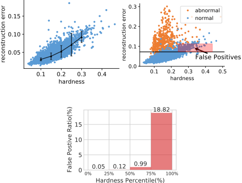
- There is a positive correlation between hardness and reconstruction error.
- There is unequal variance of reconstruction error across the range of hardness values, known as heteroscedasticity in the statistical literature.
- The higher reconstruction error of the harder normal samples encourages false positives, and conversely less hard anomalies encourages false negatives.
- This bias results in highly imbalanced false positive rates across hardness scores.
In the appendix, we show the Pearson's Correlation Coefficents between hardness and reconstruction error on various models for all datasets including tabular, time-series and image datasets. The result shows strong positive correlation especially for time-series and image datasets.
Given our definitions of hardness, the empirical result shows that an autoencoder model tends to assign higher reconstruction error to samples with higher hardness, which indicates the 'hardness bias' in these anomaly scoring models. This can lead to high false positives among normal data with high hardness, thus decreasing detection accuracy.
3.4 CADET: Calibrated Anomaly Detection
Motivation
So far, we have observed the hardness bias, whereby harder samples tend to receive higher reconstruction errors, leading to false positives. Our calibration framework aims to mitigate this problem by calibrating or 'adjusting' the scores, to adjust for the influence of hardness. Intuitively, we do this by conditioning on hardness: that is, evaluating a sample x with respect to the distribution of error conditional on hardness, P(Err(x) | H(x)).
The idea of our calibration is illustrated in Figure 1. Before calibration (Figure 1, left), the distribution of reconstruction errors varies significantly with hardness, and therefore the harder samples are more likely to be false positives. Our approach (right) calibrates the scores by mapping them into a consistent distribution that can be more fairly compared across different hardness values, leading to more accurate predictions and more meaningful anomaly scores.
Overview
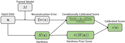
Figure 4 shows the overall framework for our approach. A key design choice of our framework is its 'plug-in' nature, allowing for flexibility and efficiency by plugging in any trained anomaly detection model M : X → R into our framework. The reconstruction error Err(x) is computed by the deep model M. Our calibration framework first computes the sample hardness H(x), then uses it to calibrate the errors, i.e., adjust them for their sample hardness.
Calibration Approach
Let our training samples be x1, · · · , xn ∈ Xtrain. As input to our approach, we have our trained plug-in model M : X → R, using which we compute the plug-in model's errors:
To start the calibration process, we compute hardness values based on the null models defined in Eq. (3), (4) and (5) depending on the data type:
In general, our main idea is to learn the conditional distribution of error given hardness, P (Err(x) | H(x)), for normal data. At the test time, we will compare the empirical errors of test samples to the learned conditional distribution, to adjust for the effect of hardness.
To capture this conditional distribution, we first fit the conditional quantile ˆ q1-ε(h) of error ei, which fits the (1 - ε) quantiles of the error conditioning on hardness h for training set data (thus, the fitted ˆ q1-ε is a function with input h):
To obtain ˆ q1-ε(h), any conditional quantile estimator(CONDQUANTILE) could be used; for a simple, efficient and non-parametric approach, we use B-splines[Bartels et al., 1995].
ˆ q1-ε(h) is an estimate of the 'baseline' level of error given hardness level h for normal data. However, recall that in our empirical observations in Section 3.3 and Figure 3(top left), we observed that as hardness increases, the mean of error values increased with unequal variance or spread. This suggests that in addition to fitting the conditional quantile ˆ q1-ε(h), we should also fit an estimate of the conditional spread ˆσ(h), which can be any estimator of the spread of the error distribution at hardness level h. In our case, we use the conditional inter-quartile range (IQR): the IQR is a standard measure defined as the difference between the 75% and 25% quantiles of the distribution, and provides a robust measure of the distribution spread. Hence, we fit two additional conditional quantiles at the 0.75 and 0.25 levels and take their difference:
Next, we define our calibrated anomaly score. Consider a (training or test) sample x, with hardness H(x). Starting with its (uncalibrated) error Err(x), we calibrate this by subtracting the conditional quantile ˆ q1-ε(H(x)) and dividing the result by the conditional spread ˆσ(H(x)), giving the first term in Eq. (10).
Considering the intrinsic imbalanced distribution of hardness values, we introduce the second term π(H(x)) in Eq. (10), a hardness prior score, which captures the normal distribution of hardness values H(x) in the training set: for simplicity, we fit a Gaussian to the hardness values in the training set. Then, given the sample x, we add the absolute value of its z-score (i.e., no. of standard deviations away from the mean) of this Gaussian (denoted π(H(x))) as part of the anomaly score, along with a weight hyperparameter λ > 0 to adjust its scale relative to the first term.
Definition 3.1 (Calibrated Anomaly Score). Given a (training or test) sample x ∈ X, its calibrated anomalousness score is:
Calibrated Decision Rule
To provide a basis for decision making in real-world applications, our decision rule Dε outputs a binary decision of 1 if the point is an anomaly, and 0 otherwise. Since false positives are often costly, Dε allows for a user-given probabilistic threshold of ε, designating that its false positive rate should be bounded by ε.
Our approach for obtaining this guarantee is based on conformal prediction [Vovk et al., 2005], a simple and modelagnostic statistical approach for obtaining confidence guarantees in finite-sample and distribution-free settings. This framework relies on conformity scores quantifying the error made for a given input - in our case, we consider the pairs (H(x), Err(x)), and the conformity score is the calibrated anomaly score s(x) in Definition 3.1.
To apply this framework, we define a calibration set Xcal, which can be either a validation set separate from the training data, or (if this is unavailable) the training set. Using a validation set allows for theoretical guarantees (Theorem 1). However, we want our framework to be usable even when M is pre-trained; in this case, the full training set is often used for training without a separate validation set available. For this case, we show in our experiments that even using the training set as Xcal can still provide well-calibrated decision rules in practice.
Let m be the number of samples in Xcal. We sort the values {s(x) : x ∈ Xcal}, and define ˆQ1-ε as the ⌈(m+1)(1-ε)⌉th smallest value in this set. Then, the decision rule Dε(x) can be defined by treating ˆQ1-ε as a threshold:
Algorithm 1 summarizes our approach.
Algorithm 1: CADET: Calibrated Anomaly Detection
Input : Training set Xtrain, Calibration set Xcal, Test set Xtest, Threshold ε, Trained plug-in model M, Prior weight λ > 0 Output: Anomalousness score s(x) and decision Dε(x) ∈ {0, 1} 1 Compute errors: ei = Err(xi) for xi ∈ Xtrain Using Eq. (6) 2 Compute hardness: hi = H(xi) for xi ∈ Xtrain Using Eq. (7) 3 Fit conditional quantile ˆ q1-ε(h) and spread ˆσ(h) Using Eq. (8), (9) 4 Calibrated scores: s(x) := Err(x)-ˆ q1-ε(H(x)) ˆσ(H(x)) +λ · π(H(x)) for x ∈ Xcal Def. 3.1 5 Threshold: ˆQ1-ε := ⌈(m+ 1)(1 - ε)⌉th smallest value in {s(x) : x ∈ Xcal} 6 Apply ε-level decision rule on x inXtest : 7 Dε(x) = {1 if s(x) > ˆQ1-ε 0 otherwise Using Eq. (11)False Positive Guarantee
This conformal prediction framework allows us to obtain guarantees on the false positive rate of this decision procedure.
Theorem 1 (Bound of False Positive Probability). Given the decision rule Dε and a (non-anomalous) test sample x, the false positive probability is bounded as:
where the probability is taken over the randomness in x and the calibration data ˜x1, · · · , ˜xm ∈ Xcal, where we use a validation set as calibration data.
Proof. Our proof follows the standard techniques used in the conformal literature [Vovk et al., 2005; Romano et al., 2020], particularly, the use of exchangeability. The full proof can be found in our Supplementary Material.
4 Experiments
We conduct experiments to answer the following research questions:
- RQ1 (Generality & Efficiency): Can our calibration method improve the accuracy of different pre-trained deep anomaly detection techniques? How efficient is the calibration method?
- RQ2 (Accuracy & Ablation Study): Does our method outperform baseline methods in accuracy of anomaly detection in different datasets?
- RQ3 (Probabilistic Guarantees): Can our method give an approximate false positive guarantee in anomaly detection?
| AE | VAE | DAE | RealNVP | |||||
|---|---|---|---|---|---|---|---|---|
| Datasets | Base | CADET | Base | CADET | Base | CADET | Base | CADET |
| OPTDIGITS | 0.957 | 0.971 | 0.872 | 0.863 | 0.959 | 0.969 | 0.916 | 0.921 |
| PENDIGTIS | 0.972 | 0.978 | 0.923 | 0.956 | 0.991 | 0.994 | 0.995 | 0.996 |
| SATELLITE | 0.845 | 0.887 | 0.816 | 0.859 | 0.838 | 0.882 | 0.832 | 0.881 |
| SATIMAGE-2 | 0.996 | 0.998 | 1.000 | 1.000 | 0.997 | 1.000 | 0.999 | 1.000 |
| VERTEBRAL | 0.595 | 0.630 | 0.482 | 0.624 | 0.645 | 0.632 | 0.649 | 0.673 |
| MSL | 0.594 | 0.641 | 0.537 | 0.633 | 0.593 | 0.637 | 0.589 | 0.632 |
| SMAP | 0.597 | 0.654 | 0.581 | 0.653 | 0.592 | 0.645 | 0.578 | 0.630 |
| MNIST | 0.958 | 0.984 | 0.930 | 0.964 | 0.927 | 0.985 | 0.531 | 0.732 |
| F-MNIST | 0.919 | 0.944 | 0.899 | 0.913 | 0.887 | 0.924 | 0.639 | 0.726 |
4.1 Experimental Setup
The experiments are conducted for AE, VAE and other variant models on publicly available image, time series and tabular datasets. We use Area Under Curve (AUC) metric for evaluation to avoid threshold setting. The train-test split settings are the same for the baselines and our methods.
Full details about datasets, baseline settings, model architectures, hyperparameters, ablation study, etc. can be found in our Supplementary Material.
4.2 RQ1. Generality &Efficiency
To evaluate the generality of CADET, we compare the performance before and after CADET calibration on four types of models and different datasets in Table 1. CADET improves the accuracy in almost all cases, often substantially.
Besides, all these improvements come at very low computational cost: as presented in our Supplementary Material, the longest running time across all datasets and methods was 1.31s for both the hardness and calibration steps.
4.3 RQ2. Accuracy &Ablation Study
In Table 2, we show the anomaly detection accuracy in terms of AUC score, of our CADET method on Autoencoder (AE) and the baselines, on the benchmark datasets. The results show that CADET outperforms all tested baselines in almost all cases.
In the appendix, we perform an ablation study to show the effect of each component of CADET separately: CADET with only hardness prior scores, CADET without the prior, and CADET. We find that only using prior scores performs worse than the base model for all datasets, which verifies the effectiveness of calibration. Additionally, it shows that CADET without prior scores can achieve fairly similar performance with the complete CADET for time-series, image data and most tabular data. These findings show that calibration is the essential component of our method, while the prior is auxiliary.
4.4 RQ3. Probabilistic Guarantees
To study the effectiveness of our decision rule and our method at mitigating hardness bias, we show the calibrated scores and compare the false positive rates between uncalibrated reconstruction error and calibrated scores under our decision rule in Eq. (11) with ϵ = 5% on F-MNIST.
Figure 5 (left) shows that the previously observed positive correlation between hardness and anomaly score has been removed by calibration. This results in a more balanced distrihardness bution of scores across hardness values, as compared to reconstruction error. Figure 5 (right) shows that our calibrated decision rule has a balanced 5% false positive rate across different hardness ranges, as compared to the extremely unbalanced false positive rate of reconstruction error.
| Datasets | PCA | IForest | OCSVM | DAGMM | RAPP | CADETAE |
|---|---|---|---|---|---|---|
| OPTDIGITS | 0.592 | 0.813 | 0.588 | 0.969 | 0.895 | 0.971 |
| PENDIGITS | 0.951 | 0.975 | 0.954 | 0.963 | 0.966 | 0.978 |
| SATELLITE | 0.657 | 0.774 | 0.664 | 0.787 | 0.851 | 0.887 |
| SATIMAGE-2 | 0.998 | 0.999 | 1.000 | 0.979 | 0.999 | 0.998 |
| VERTEBRAL | 0.542 | 0.494 | 0.552 | 0.460 | 0.506 | 0.630 |
| MSL | 0.612 | 0.572 | 0.628 | 0.598 | 0.635 | 0.641 |
| SMAP | 0.622 | 0.580 | 0.642 | 0.548 | 0.643 | 0.654 |
| MNIST | 0.885 | 0.855 | 0.887 | 0.798 | 0.979 | 0.984 |
| F-MNIST | 0.906 | 0.919 | 0.894 | 0.854 | 0.933 | 0.944 |
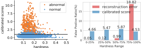
Figure 5: Left: The calibrated scores versus hardness values. Right: False Positive Rate (%) comparison between reconstruction error and calibrated score. The 1st hardness range (0 - 25%) has samples in the lowest quarter of hardness values, etc. Both methods use probabilistic threshold of ϵ = 5% as decision rule in Eq. (11).
5 Conclusion
In our work, we firstly show the hardness bias in existing anomaly detection models, where the models can assign higher anomaly scores to samples which are intrinsically harder to model. This bias leads to imbalanced false positives and accuracy degradation in practice. Therefore, we introduce the CADET framework to calibrate the original anomaly scores to adjust the effect of hardness bias in a post-hoc way. Thanks to the post-hoc property, the framework can be flexibly applied on top of the anomaly detection module with very low computational cost. The experiments show that CADET can effectively improve performance on multiple data modalities, and with four types of deep learning models. By mitigating hardness bias through calibration, CADET also provides more balanced false positive rates across hardness values compared to the original anomaly scores.
Acknowledgements
This work was supported in part by NUS ODPRT Grant R252-000-A81-133. We thank Shen Li for attentive proofreading.
@inproceedings{ijcai2022p278,
  title     = {CADET: Calibrated Anomaly Detection for Mitigating Hardness Bias},
  author    = {Deng, Ailin and Goodge, Adam and Ang, Lang Yi and Hooi, Bryan},
  booktitle = {Proceedings of the Thirty-First International Joint Conference on
               Artificial Intelligence, {IJCAI-22}},
  publisher = {International Joint Conferences on Artificial Intelligence Organization},
  editor    = {Luc De Raedt},
  pages     = {2002--2008},
  year      = {2022},
  month     = {7},
  note      = {Main Track},
  doi       = {10.24963/ijcai.2022/278},
  url       = {https://doi.org/10.24963/ijcai.2022/278},
}
TY - CPAPER TI - CADET: Calibrated Anomaly Detection for Mitigating Hardness Bias AU - Deng, Ailin AU - Goodge, Adam AU - Ang, Lang Yi AU - Hooi, Bryan T2 - Proceedings of the Thirty-First International Joint Conference on Artificial Intelligence, IJCAI-22 PB - International Joint Conferences on Artificial Intelligence Organization PY - 2022 SP - 2002 EP - 2008 DO - 10.24963/ijcai.2022/278 UR - https://doi.org/10.24963/ijcai.2022/278 ER -Copied
Machine-readable versions of this paper, for tools and AI agents:





