
Long-term Spatio-Temporal Forecasting via Dynamic Multiple-Graph Attention
Proceedings of the Thirty-First International Joint Conference on Artificial Intelligence. Main Track. Pages 2225-2232.
https://doi.org/10.24963/ijcai.2022/309
Keywords
- Data Mining: Mining Spatial and/or Temporal Data
- Multidisciplinary Topics and Applications: Smart Cities
Abstract
Many real-world ubiquitous applications, such as parking recommendations and air pollution monitoring, benefit significantly from accurate long-term spatio-temporal forecasting (LSTF). LSTF makes use of long-term dependency structure between the spatial and temporal domains, as well as the contextual information. Recent studies have revealed the potential of multi-graph neural networks (MGNNs) to improve prediction performance. However, existing MGNN methods do not work well when applied to LSTF due to several issues: the low level of generality, insufficient use of contextual information, and the imbalanced graph fusion approach. To address these issues, we construct new graph models to represent the contextual information of each node and exploit the long-term spatio-temporal data dependency structure. To aggregate the information across multiple graphs, we propose a new dynamic multi-graph fusion module to characterize the correlations of nodes within a graph and the nodes across graphs via the spatial attention and graph attention mechanisms. Furthermore, we introduce a trainable weight tensor to indicate the importance of each node in different graphs. Extensive experiments on two large-scale datasets demonstrate that our proposed approaches significantly improve the performance of existing graph neural network models in LSTF prediction tasks.
- [Bruna et al., 2013] Joan Bruna, Wojciech Zaremba, Arthur Szlam, and Yann LeCun. Spectral Networks and Lo- cally Connected Networks on Graphs. arXiv preprint arXiv:1312.6203, 2013.
- [Chai et al., 2018] Di Chai, Leye Wang, and Qiang Yang. Bike Flow Prediction with Multi-Graph Convolutional Networks. In Proceedings of the 26th ACM SIGSPATIAL international conference on advances in geographic infor- mation systems, pages 397-400, 2018.
- [Defferrard et al., 2016] Michaël Defferrard, Xavier Bres- son, and Pierre Vandergheynst. Convolutional Neural Net- works on Graphs with Fast Localized Spectral Filtering. In Proceedings of the 30th International Conference on Neural Information Processing Systems, NIPS'16, pages 3844-3852, Dec. 2016.
- [Geng et al., 2019] Xu Geng, Yaguang Li, Leye Wang, Lingyu Zhang, Qiang Yang, Jieping Ye, and Yan Liu. Spa- tiotemporal Multi-Graph Convolution Network for Ride- Hailing Demand Forecasting. In Proceedings of the AAAI conference on artificial intelligence, volume 33, pages 3656-3663, 2019.
- [Guo et al., 2019] Shengnan Guo, Youfang Lin, Ning Feng, Chao Song, and Huaiyu Wan. Attention based spatial- temporal graph convolutional networks for traffic flow forecasting. In Proceedings of the AAAI Conference on Ar- tificial Intelligence, volume 33, pages 922-929, 07 2019.
- [Huang et al., 2020] Rongzhou Huang, Chuyin Huang, Yubao Liu, Genan Dai, and Weiyang Kong. LSGCN: Long Short-Term Traffic Prediction with Graph Convo- lutional Networks. In Proceedings of the Twenty-Ninth International Joint Conference on Artificial Intelligence, IJCAI-20, pages 2355-2361, Jul. 2020. IJCAI
- [Li et al., 2018] Yaguang Li, Rose Yu, Cyrus Shahabi, and Yan Liu. Diffusion Convolutional Recurrent Neural Net- work: Data-Driven Traffic Forecasting. arXiv preprint arXiv:1707.01926, Feb. 2018.
- [Liu et al., 2021] Chang Liu, Hairui Zhang, Zhen Cheng, Juanyong Shen, Junhao Zhao, Yichao Wang, Shuo Wang, and Yun Cheng. Emulation of an atmospheric gas- phase chemistry solver through deep learning: Case study of chinese mainland. Atmospheric Pollution Research, 12(6):101079, 2021.
- [Lv et al., 2020] Mingqi Lv, Zhaoxiong Hong, Ling Chen, Tieming Chen, Tiantian Zhu, and Shouling Ji. Temporal Multi-Graph Convolutional Network for Traffic FlowPre- diction. IEEE Transactions on Intelligent Transportation Systems, pages 1-12, May. 2020.
- [Shao et al., 2017] Wei Shao, Flora D Salim, Tao Gu, Ngoc- Thanh Dinh, and Jeffrey Chan. Traveling Officer Problem: Managing Car Parking Violations Efficiently Using Sen- sor Data. IEEE Internet of Things Journal, 5(2):802-810, 2017.
- [Shuman et al., 2013] David I Shuman, Sunil K. Narang, Pascal Frossard, Antonio Ortega, and Pierre Van- dergheynst. The emerging field of signal processing on graphs: Extending high-dimensional data analysis to net- works and other irregular domains. IEEE Signal Process- ing Magazine, 30(3):83-98, 2013.
- [Van Erven and Harremos, 2014] Tim Van Erven and Peter Harremos. Rényi divergence and kullback-leibler di- vergence. IEEE Transactions on Information Theory, 60(7):3797-3820, 2014.
- [Wang et al., 2020a] Senzhang Wang, Hao Miao, Hao Chen, and Zhiqiu Huang. Multi-task adversarial spatial-temporal networks for crowd flow prediction. In Proceedings of the 29th ACM international conference on information & knowledge management, pages 1555-1564, 2020.
- [Wang et al., 2020b] Shuo Wang, Yanran Li, Jiang Zhang, Qingye Meng, Lingwei Meng, and Fei Gao. Pm2.5-gnn: A domain knowledge enhanced graph neural network for pm2.5 forecasting. In Proceedings of the 28th Interna- tional Conference on Advances in Geographic Information Systems, SIGSPATIAL '20, page 163-166, 2020.
- [Wang et al., 2021] Chunyang Wang, Yanmin Zhu, Tianzi Zang, Haobing Liu, and Jiadi Yu. Modeling inter-station relationships with attentive temporal graph convolutional network for air quality prediction. In Proceedings of the 14th ACM International Conference on Web Search and Data Mining, WSDM '21, page 616-634, 2021.
- [Wen et al., 2019] Congcong Wen, Shufu Liu, Xiaojing Yao, Ling Peng, Xiang Li, Yuan Hu, and Tianhe Chi. A novel spatiotemporal convolutional long short-term neural net- work for air pollution prediction. Science of the total envi- ronment, 654:1091-1099, 2019.
- [Wu et al., 2019] Zonghan Wu, Shirui Pan, Guodong Long, Jing Jiang, and Chengqi Zhang. Graph wavenet for deep spatial-temporal graph modeling. In Proceedings of the Twenty-Eighth International Joint Conference on Artificial Intelligence, IJCAI-19, pages 1907-1913, 7 2019. IJCAI
- [Yu et al., 2018] Bing Yu, Haoteng Yin, and Zhanxing Zhu. Spatio-Temporal Graph Convolutional Networks: A Deep Learning Framework for Traffic Forecasting. In Proceed- ings of the 27th International Joint Conference on Artifi- cial Intelligence, pages 3634-3640, 2018. IJCAI
- [Zhang et al., 2020a] Weijia Zhang, Hao Liu, Yanchi Liu, Jingbo Zhou, and Hui Xiong. Semi-Supervised Hierarchi- cal Recurrent Graph Neural Network for City-Wide Park- ing Availability Prediction. In Proceedings of the AAAI Conference on Artificial Intelligence, volume 34, pages 1186-1193, 2020.
- [Zhang et al., 2020b] Xu Zhang, Ruixu Cao, Zuyu Zhang, and Ying Xia. Crowd Flow Forecasting with Multi-Graph Neural Networks. In 2020 International Joint Conference on Neural Networks (IJCNN), pages 1-7, Jul. 2020.
- [Zheng et al., 2020] Chuanpan Zheng, Xiaoliang Fan, Cheng Wang, and Jianzhong Qi. Gman: A graph multi- attention network for traffic prediction. In Proceedings of the AAAI Conference on Artificial Intelligence, volume 34, pages 1234-1241, 2020.
References were extracted automatically from the PDF and may contain errors.
Full text extracted automatically from the PDF; figures, tables and equations may differ. The PDF is the version of record.
1 Introduction
Recently, various spatio-temporal prediction tasks have been investigated, including traffic flow [Li et al., 2018; Huang et al., 2020; Yu et al., 2018], parking availability [Zhang et al., 2020a], and air pollution [Wang et al., 2020b; Wen et al., 2019; Liu et al., 2021]. All the scenarios above benefit from an accurate forecast by leveraging historical data in the long run, namely, long-term spatio-temporal forecasting (LSTF).
†Equal contribution.
∗Corresponding authors.
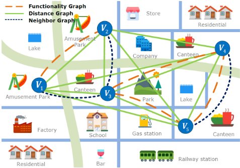
One main challenge in LSTF is to effectively capture the long-term spatio-temporal dependency and extract contextual information. Recently, multi-graph neural networks (MGNNs) [Wang et al., 2021] have received increasing attention for spatio-temporal forecasting problems. Specifically, as shown in Figure 1, each node's value Vi is estimated in the long run using historical data and correlations across nodes of a distance graph, where each edge denotes the correlation or dependency between two different nodes. Furthermore, the functionality similarities of surrounding areas, which represent contextual information, can also be used for prediction purposes. Compared to the single graph approach, which may not comprehensively capture all the relationships, the MGNN-based approach is appropriate for leveraging more information and features by integrating different graphs. Thus, in this work, we choose the MGNNbased approach to infer how information about each node evolves over time.
Although MGNNs show potential for extracting contextual information around prediction sites, four significant limitations remain when solving the LSTF problem:
- Most existing MGNN studies consider only the spatial similarity of nodes, such as the distance similarity and neighborhood correlation. Previous studies have shown that the distance similarity is insufficient to represent correlations among nodes with spatio-temporal attributes [Geng et al., 2019]. Wu et al. [Wu et al., 2019] proposed an adaptive adjacency matrix to discover hidden spatial dependencies directly from historical records of each node in an end-to-end fashion by computing the inner product of the nodes' learnable embedding. However, these works did not utilize well the existing prior knowledge encoded as an adjacency matrix, which may result in missing vital information.
- Fusing different graph models is challenging. For multi-graph-based problems, the graph models differ with different scales; thus, it is inappropriate to simplymerge them using weighted sum or other averaging approaches. Additionally, how to align each node in different graphs is challenging since nodes in different graphs are associated with different spatio-temporal information.
- Existing multi-graph fusion approaches rely heavily on specific models. The current MGNNs lack generalizability. Specifically, the existing graph construction approaches and fusion methods need to be strictly bonded, assuming specific graph neural network structures. Although such an end-toend framework provides a convenient method, it induces various difficulties in examining the importance of each graph to find a better combination of each module.
- Long-term spatio-temporal dependency is not considered. Usually, MGNNs tend to learn the spatio-temporal dependency by projecting mapping from data within the observation window and the prediction horizon. However, due to the limitation of data sources, existing graph models, such as the distance graph [Li et al., 2018] or the neighbor graph [Geng et al., 2019] represent only the static spatial information, which cannot capture the long-term spatio-temporal dependency.
To address the issues above, we investigate graph construction and fusion mechanisms, and make improvements to each component. Specifically, we take advantage of human insights to build a new graph model namely 'heuristic graph', which can represent the long-range distribution of the collected spatio-temporal data. Aiming to align various graphs with different information, we then employ the spatial and graph attention mechanisms to integrate nodes in the same graph and different graphs. Furthermore, to dynamically capture the contextual information and temporal dependency of each node in different graphs, we construct an adaptive correlation tensor to indicate the importance of each node. In summary, the main contributions of this paper are as follows:
- We propose a new graph model namely 'heuristic
- graph', for the LSTF problem, which can represent the long-term spatio-temporal dependency from historical data or human insights and can be widely used for various graph neural networks.
- We design a novel graph model fusion module called a dynamic graph fusion block to integrate various graph models with graph attention and spatial attention mechanisms, aiming to align nodes within graphs and across different graphs. We further construct a learnable weight tensor for each node to flexibly capture the dynamic correlations between nodes.
- We conduct extensive experiments on two large-scale public real-world spatio-temporal datasets. We validate the effectiveness of the proposed new graph models and fusion approaches using ablation studies.
2 Methodologies
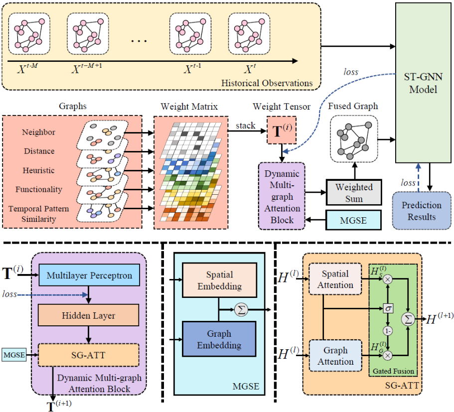
As shown in Figure 2, the proposed framework consists of three major components: the graph construction module, the dynamic multi-graph fusion module, and the spatio-temporal graph neural network (ST-GNN). We designed five graphs to represent different aspects of the spatio-temporal information in the graph construction module. In the dynamic multi-graph fusion module, we align spatial and temporal dependency using an adaptive trainable tensor and introduce graph and spatial attention mechanisms to calculate the correlations among nodes located in different graphs. We then obtain the prediction results with existing ST-GNN models.
2.1 Graph Construction
In this section, we describe in detail two new graph models we proposed named the heuristic graph GH = {V, E,W H } and the functionality graph GF = {V,E,W F }, combined with other three existing graphs, the distance graph GD = {V,E,W D }, neighbor graph GN = {V,E,W N }, and temporal pattern similarity graph GT = {V, E, W T }, into a multiple graph set G = {GD , GN , GF , GH , GT }.
Distance Graph. The element of distance matrix W D is defined with a thresholded Gaussian kernel as follows [Shuman et al., 2013]:
where dij is the Euclidean distance between vi and vj. ε and σ2D are used to control the sparsity and distribution of W D .
Neighbor Graph. The element of neighbor matrix W N is defined as follows:
Functionality Graph. Usually, places with similar functionalities or utilities, such as factories, schools, and hospitals, have strong correlations. In this paper, different from the functionality graph proposed by [Geng et al., 2019], we propose a new functionality graph using Pearson correlation coefficients to capture the global contextual function similarity. Denote the total number of functions is K; then the vector of the number of these functions of vertex vi is denoted as Fi = {fi,1, fi,2, · · · , fi,k, · · · , fi,K}. The functionality matrix can be obtained using Pearson correlation coefficients [Zhang et al., 2020b] by
Note that we consider all functions that contribute equally to the relationships of nodes.
Heuristic Graph. To leverage heuristic knowledge and human insights, we propose a new graph model called the heuristic graph. We create a histogram to represent the overview of the spatio-temporal training data, where each bin indicates a predefined temporal range, and the bar height measures the number of data records that fall into each bin. Then we apply a function f(x) = αe-βx to approximate the histogram. For a vertex vi, we can obtain its fitted parameters αi and βi. The distribution distance is calculated using the Euclidean distance dHij = √(α1 -α2)2 + (β1 -β2)2 . The element of the heuristic matrix W H can be defined as follows:
where σ2H is a parameter to control the distribution of W H . Kullback-Leibler (KL) divergence [Van Erven and Harremos, 2014] can be also used to create this graph, which usually quantifies the difference between two probability distributions.
Temporal Pattern Similarity Graph. For a vertex vi, the vector of the time-series data used for training is described as
Algorithm 1 Dynamic Multi-graph Fusion
Input: Weight matrices: W D , W N , W F , W H , W T
Parameter: Number of batches: Bt
Output: Fused weight matrix W ∗
- 1: Stack weight matrices to tensor T(0) ∈ R|G|×N×N .
- 2: Train T(0) while training ST-GNNmodels.
- 3: for i ∈ [0,Bt -1] do
- 4: T(i+1) ←- T(i)
- 5: i = i +1
- 6: W ∗ jk = ∑|G| i=1 T(i) (i, j, k), where W ∗ jk is the element of the weight matrix of the fused graph.
- 7: end for
- 8: returnW ∗
Ti = {ti,1, ti,2, · · · , ti,p, · · · , ti,P}, where P is the length of the series, and ti,p is the time-series data value of the vertex vi at time step p. We also use the Pearson correlation coefficients [Zhang et al., 2020b] to define the elements of the temporal pattern similarity matrix W T as follows:
2.2 Dynamic Multi-graph Fusion
The graph fusion approach plays a key role in multi-graph neural networks as multi-graphs cannot simply be merged with the average sum or the weighted sum [Wang et al., 2020a]. In this paper, a dynamic graph fusion method is proposed; the whole process of this method is shown in Figure 2 and Algorithm 1. We construct a trainable weight tensor as the input of a dynamic multi-graph attention block (DMGAB). Moreover, we incorporate the spatial and graph information into multi-graph spatial embedding (MGSE) and add this embedding to the DMGAB. To facilitate the residual connection, all layers of the DMGAB produce outputs of D dimensions, and the block can be expressed as DMGAB ∈ R|G|×N×D .
Multi-graph Spatial Embedding
We apply the spatial embedding ES vi ∈ RD to preserve the graph structure information. To represent the relationships of the nodes in different graphs, we further propose graph embedding to encode five graphs into R|G| . Then we employ a two-layer fully-connected neural network to transform the graphs into a vector RD and obtain the multi-graph embedding EMG Gi ∈ RD , where Gi is any graph. To obtain the vertex representations among multiple graphs, we fuse the spatial embedding and the multi-graph embedding as the multigraph spatial embedding (MGSE) with Evi,Gi = ES vi +EMG Gi .
Dynamic Multi-graph Attention Block
Any node in a graph is impacted by other nodes with different levels. When acting on multiple graphs, these impacts are magnified. To model inner node correlations, we design a multi-graph attention block to adaptively capture the correlations among the nodes. As shown in Figure 2, the multi-graph attention block contains spatial attention and graph attention.
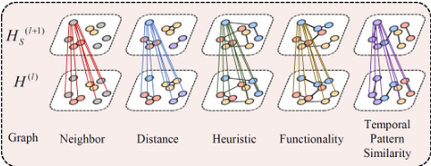
(a) spatial attention
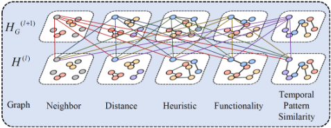
(b) graph attention
Figure 3: The attention mechanisms adopted in this paper.
We denote the input of the l-th block H(l) and denote the hidden state of the vertex vi on graph Gi in H(l) as h(l) vi,Gi . The output blocks of the spatial and graph attention mechanisms are denoted as H(l+1) S and H(l+1) G , respectively.
Spatial Attention. Inspired by [Zheng et al., 2020], we capture the contextual correlations of nodes by proposing a spatial attention mechanism (shown in Figure 3a). Different from the previous spatial attention mechanism, which acts on the hidden state of the batch of temporal data, our method acts on the hidden state of the weight tensor. Then we can calculate the next hidden state in the graph Gi as follows:
where Vi is all the vertices on the graph except the vi. αvi,vk is the attention score respecting the importance of vk to vi.
In the real world, the vertices are influenced not only by other vertices on the same graph but also other graphs. For example, the parking occupancy rate of one place is affected not only by the distance from another place but also by the functionality of another place. To this end, we concatenate the hidden state with MGSE to extract both the spatial and graph features and employ the scaled dot-product approach to calculate the relevance between vi and vk with
where ‖ is the concatenation operation and 〈·|·〉 is the inner product operation. Then svi,vk is normalized by the softmax function αvi,vk = exp (svi,vk ) / ∑vk∈Vi exp (svi,vk ). To stabilize the learning process, we concatenate M parallel attention mechanisms to extend them to the multi-head attention mechanism [Zheng et al., 2020] with
where f (m) s,1 (·), f (m) s,2 (·), and f (m) s,3 (·) are different ReLU functions serving as nonlinear projections in m-th head attention. α(m) vi,vn is calculated with a softmax function in the m-th head attention and hs(l+1) vi,Gi is the hidden state of vi ∈ Gi.
Graph Attention. We employ graph attention to obtain the self-correlations of a node in different graphs (as shown in Figure 3b). Similar to the spatial attention mechanism, we concatenate the hidden state with MGSE and employ the multi-head method to calculate the correlations. For vi, the correlation between graph Gj and Gk is defined as:
where β(m) Gj,Gk calculated with a softmax function is the attention score in the m-th head, indicating the importance of graph Gk to Gj, f (m) G,1 (·), f (m) G,2 (·), and f (m) G,3 (·) are the ReLU functions in m-th head attention.
Gated Fusion. To further extract the correlations of nodes on different graphs, we adopt the gated fusion method [Zheng et al., 2020] to consider both effects. The spatial attention H(l) S and the graph attention H(l) G in the l-th block are fused with
where the gate z is calculated by:
where Wz,1 ∈ RD×D , Wz,2 ∈ RD×D , and bz ∈ RD are the learnable parameters, ⊙ indicates the element-wise Hadamard product, and σ(·) is the sigmoid activation function. By combining the spatial and graph attention mechanisms, we further create a spatial-graph attention (SG-ATT) block, which is shown in Figure 2.
3 Experiments
3.1 Datasets
Parking: The Melbourne parking dataset, collected by the Melbourne City Council in 2019, contains 42, 672, 743 parking events recorded by the in-ground sensors every five minutes located in the Melbourne Central Business District (CBD) [Shao et al., 2017]. All sensors have been classified into 40 areas.
Air Quality: The Ministry of Ecology and Environment of China (MEE) published a large-scale air quality dataset [Wang et al., 2020b], comprising 92 air quality monitoring stations, to assess the hourly PM2.5 concentration in Jiangsu province in 2020.
3.2 Experimental Details
Baselines. We selected five state-of-the-art ST-GNN models as baselines: STGCN [Yu et al., 2018], ASTGCN [Guo et al., 2019], MSTGCN [Guo et al., 2019], ST-MGCN [Geng et al., 2019], and Graph WaveNet [Wu et al., 2019].
Platform. All experiments were trained and tested on a Linux system (CPU: Intel(R) Xeon(R) Gold 6240 CPU @2.60GHz, GPU: NVIDIA GeForce RTX 2080 Ti).
Hyper-parameters. All the tests used a 24-time step historical time window, and the prediction horizons ranged from three to 24 steps. The proposed methods were optimized with the Adam optimizer. The learning rate was set to 1e-4 . The L1 loss function was adopted to measure the performance of the proposed model. The batch size was 32, and the global seed was set to 0 for the experiment repeat. All the tests were trained for 40 epoches. The number of attention heads M and the dimension d of each attention head were set to 8 and 8 in the Parking dataset and set to 24 and 6 in the Air Quality dataset.
Evaluation Metrics. In our study, mean absolute error (MAE) and root mean square error (RMSE) were used.
3.3 Results and Analysis
Table 1 summarizes the results of all ST-GNN models based on the two datasets. The prediction horizon ranged from three time steps to 24 steps. The best evaluation results are highlighted in boldface. The number of highlighted values is also recorded (i.e., the winning counts) to compare the performance of different models.
In the first experiment, we aimed to provide an overall evaluation of the performance of the constructed graphs and the fusion approaches. We compared results between the existing ST-GNN without the proposed fused multi-graphs, and the results with the proposed multi-graph mechanism.
Table 1 shows the following: (1) When the proposed dynamic multi-graph fusion approach (marked with '*') was used, the prediction performances significantly improved. For example, when the STGCN method was used, our method had an average RMSE decrease of 9.5% (over all prediction horizons). This indicates that our multi-graph fusion methods can extract more information and are effective for various ST-GNN models. (2) When the same ST-GNN methods are used, our proposed methods outperform the original ones in winning counts under all circumstances, which demonstrates the strong generality of our approach. (3) The results illustrate that our model is more suitable for the LSTF problem. Specifically, with the increase in prediction horizons, the gaps between vanilla ST-GNN models and our proposed models become larger. Figure 4 illustrates the trends of the proposed model and existing ST-GNN models with various prediction horizons. We found that the performance of the proposed models (green line) did not show a significant drop with the increasing prediction horizons while existing ST-GNN models (red line) underperformed in a long-run prediction.
| Datasets | Methods Metric | STGCN | STGCN* | ST-MGCN* | ASTGCN | ASTGCN* | MSTGCNMSTGCN* | Graph WaveNet | Graph WaveNet* | |||
|---|---|---|---|---|---|---|---|---|---|---|---|---|
| Parking | RMSE | 3 6 9 12 15 18 21 | 0.0514 0.0658 0.0787 0.0903 0.1007 0.1105 | 0.1194 | ST-MGCN 0.0553 0.0677 0.0794 0.0900 0.0999 0.1092 0.1178 0.1259 0.0376 0.0467 0.0556 | 0.0524 | 0.0517 0.0642 0.0748 0.0843 0.1115 | 0.0493 0.0611 0.0702 0.0776 0.0850 | 0.0604 0.0724 0.0833 0.0939 0.1041 0.1140 | 0.0479 0.0607 | 0.0477 0.0608 0.0709 | 0.0473 0.0594 0.0684 0.0762 0.0832 0.0893 |
| 0.0607 | 0.0646 | |||||||||||
| 0.0751 0.0869 | 0.0748 | 0.0706 | ||||||||||
| 0.0992 | 0.0839 | 0.0796 | 0.0801 | |||||||||
| 0.1107 | 0.0924 | 0.0875 0.0947 | 0.0883 0.0965 | |||||||||
| 0.1210 | 0.1002 | 0.1228 | 0.0915 | |||||||||
| 0.1301 | 0.1075 | 0.1308 | 0.0977 | 0.1229 | 0.1017 | 0.1040 | 0.0946 | |||||
| 24 | 0.1393 | 0.1276 | 0.1143 | 0.1410 | 0.1035 | 0.1318 | 0.1071 | 0.1114 | 0.0996 | |||
| MAE | 3 0.0425 | 0.0358 | 0.0360 | 0.0362 | 0.0342 | 0.0443 | 0.0328 | 0.0323 | 0.0321 | |||
| 6 | 0.0529 | 0.0457 | 0.0450 | 0.0452 | 0.0431 | 0.0532 | 0.0424 | 0.0422 | 0.0416 | |||
| 9 | 0.0616 | 0.0555 | 0.0529 | 0.0531 | 0.0504 | 0.0613 | 0.0502 | 0.0499 | 0.0485 | |||
| 12 15 | 0.0711 | 0.0640 | 0.0638 | 0.0600 | 0.0601 | 0.0565 | 0.0692 | 0.0575 0.0637 | 0.0571 0.0635 | 0.0545 0.0599 | ||
| 18 | 0.0798 0.0882 | 0.0719 0.0795 | 0.0715 0.0788 | 0.0667 0.0728 | 0.0675 0.0742 | 0.0623 0.0674 | 0.0769 0.0846 | 0.0695 | 0.0698 | 0.0646 | ||
| 0.0866 | 0.0855 | 0.0786 | 0.0810 | 0.0722 | 0.0918 | 0.0752 | 0.0755 | 0.0687 | ||||
| 21 | 0.0956 | 0.0768 | 0.0995 | 0.0794 | 0.0812 | |||||||
| 24 | 0.1036 | 0.0934 | 0.0919 | 0.0841 | 0.0867 | 0.0724 | ||||||
| Quality | RMSE | 3 6.6843 | 6.3609 | 6.7802 | 6.3255 | 6.3958 | 6.9846 | 7.0427 | 6.3729 | 6.4878 | 6.1353 | |
| 6 8.3989 | 7.7995 | 8.7083 | 7.6470 | 7.7519 | 8.1628 | 8.4449 | 7.6549 | 8.2323 | 8.5556 | |||
| 9 10.8079 | 9.7762 | 8.6881 | 10.3522 | 8.6431 | 9.0522 10.7794 | 9.4715 10.2963 | 9.3188 10.7145 | 8.7717 9.6747 | 10.3232 12.9487 | 10.8160 13.1379 | ||
| 12 15 | 11.7172 10.1575 | 9.5392 | 11.5615 12.3340 | 9.5453 10.3465 | 11.9669 | 10.9218 | 11.4235 | 10.7134 | 15.7093 | 15.0418 | ||
| 18 | 11.9014 10.4241 | 12.7944 | 10.9299 | 13.2015 | 11.8600 | 12.3950 | 11.1146 | 19.2235 | 14.1381 | |||
| 21 | 11.3408 | 13.1333 | 11.2794 | 14.4416 | 11.6768 | 13.1675 | 10.7613 | 21.1240 | ||||
| 24 | 12.5268 | 13.4125 | ||||||||||
| 12.9587 | 11.8283 | 13.4853 | 11.3442 | 14.6537 | 10.7624 | 13.3226 | 11.3835 | 21.2758 | 13.2053 | |||
| Air | MAE | 3 4.8973 | 4.5597 | 5.2823 | 4.5859 | 4.7643 | 5.4481 | 5.3349 | 4.7283 | 4.9826 | 4.4299 | |
| 6.9107 | 6.0212 | 7.1787 | 5.7940 | 6.0111 | 6.5127 | 6.7291 | 5.9757 | 6.6243 | 6.8427 | |||
| 6 9 | 7.7049 | 6.9780 | 8.8038 | 6.7984 | 7.2884 | 7.8179 | 7.6316 | 7.0500 | 8.6868 | 8.9678 | ||
| 12 | 8.8756 | 7.9221 | 9.9872 | 7.7235 | 9.1761 | 8.6078 | 9.1154 | 7.9514 | 11.1945 | 11.0713 | ||
| 15 | 9.3082 | 8.5626 | 10.7280 | 8.5209 | 10.3348 | 9.1881 | 9.8296 | 9.0196 | 13.6732 | 12.3349 | ||
| 18 | 10.2937 | 8.8195 | 11.1683 | 9.0835 | 11.5575 | 9.0804 | 10.7857 | 9.3868 | 16.5516 | 11.8929 | ||
| 21 | 10.7669 | 9.7565 | 11.4962 | 9.4271 | 12.7541 | 8.8657 | 11.5581 | 8.9675 | 18.0054 | 11.1300 | ||
| 24 | 10.9152 | 10.2256 | 11.8230 | 9.5085 | 12.9317 | 8.9076 | 11.6787 | 9.6138 | 18.1966 | 10.8037 | ||
| Count | 0 | 32 | 0 | 32 | 6 | 26 | 0 | 32 | 5 | 27 | ||
| Model | STGCN | ASTGCN | MSTGCN | ST-MGCN | Graph WaveNet | ||
|---|---|---|---|---|---|---|---|
| 12 | † ‡ | 0.0648 0.0640 | 0.0648 0.0565 | 0.0579 0.0575 | 0.0612 0.0599 | 0.0579 0.0545 | |
| MAE | 24 | † ‡ | 0.0961 0.0934 | 0.0961 0.0768 | 0.0809 0.0794 | 0.0857 0.0836 | 0.0818 0.0724 |
| 12 | † ‡ | 0.0910 0.0903 | 0.091 0.0776 | 0.0882 0.0796 | 0.0860 0.0836 | 0.0818 0.0762 | |
| RMSE | 24 | † ‡ | 0.1306 0.1276 | 0.1178 0.1035 | 0.1099 0.1071 | 0.1281 0.1139 | 0.1129 0.0996 |
3.4 Ablation Study
To validate the performance of each component, we further conducted ablation studies on the Parking dataset.
The Performance of Functionality Graphs. Table 2 shows that (1) most ST-GNN models using the proposed functionality graph (marked with '‡') outperformed those using the functionality graph proposed by [Geng et al., 2019]. (2) The results using the proposed functionality graph showed less drop when the prediction horizons changed from 12 to 24, which suggests that our proposed functionality graph performs well in LSTF tasks.
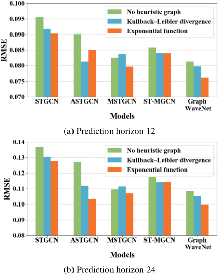
The Performance of Heuristic Graph. Figure 5 shows that graphs generated by exponential approximation function in general outperformed other approaches with prediction horizons 12 and 24, while graphs generated by the KL divergence outperformed graphs without heuristic graphs.
The Performance of SG-ATT. Figure 4 shows the performance of the framework with (marked with '∗ ') and without SG-ATT (marked with '⋆ '). We observe that the SG-ATT
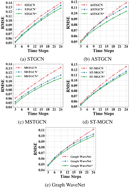
mechanism contributes considerably to the proposed framework, especially in long-term prediction.
4 RelatedWork
Graph convolution networks (GCN) attracts much attention in spatio-temporal data prediction tasks recently. Bruna et al. [Bruna et al., 2013] proposed convolutional neural networks on graphs for the first time, which Defferrard et al. [Defferrard et al., 2016] extended using fast localized convolutions. Using graph-based approaches, we can easily model spatial data. However, the observation from a single graph usually brings bias, while multiple graphs can offset and attenuate the bias. Chai et al. [Chai et al., 2018] designed a multi-graph convolutional network for bike flow prediction. Geng et al. [Geng et al., 2019] encoded non-Euclidean pairwise correlations among regions into multiple graphs and then modeled these correlations using multi-graph convolution for ride-hailing demand forecasting. Lv et al. [Lv et al., 2020] encoded non-Euclidean spatial and semantic correlations among roads into multiple graphs for traffic flow prediction. However, the relationships among graphs are ignored. Moreover, the input graphs are fixed and cannot be adapted to change during training and long-term temporal information is rarely considered.
5 Conclusion
In this paper, we try to solve the LSTF problem with multigraph neural networks. We propose two new graphs to extract heuristic knowledge and contextual information from spatiotemporal data. Specifically, we designed a heuristic graph to capture the long-term pattern of the data and a functional similarity graph to represent the similarity of functionality between two areas. To align nodes in graphs and timestamps, we designed a dynamic graph multi-graph fusion module and fed them to various graph neural networks. Extensive experiments on real-world data demonstrated the effectiveness of the proposed methods for enhancing the prediction capacity in LSTF problems. In the future, we will apply the proposed framework to additional graph-based applications.
Acknowledgments
This work was made possible, in part, by grant NPRP No. NPRP12S-0313-190348 from the Qatar National Research Fund (a member of The Qatar Foundation). The statements made herein are solely the responsibility of the authors.
@inproceedings{ijcai2022p309,
  title     = {Long-term Spatio-Temporal Forecasting via Dynamic Multiple-Graph Attention},
  author    = {Shao, Wei and Jin, Zhiling and Wang, Shuo and Kang, Yufan and Xiao, Xiao and Menouar, Hamid and Zhang, Zhaofeng and Zhang, Junshan and Salim, Flora},
  booktitle = {Proceedings of the Thirty-First International Joint Conference on
               Artificial Intelligence, {IJCAI-22}},
  publisher = {International Joint Conferences on Artificial Intelligence Organization},
  editor    = {Luc De Raedt},
  pages     = {2225--2232},
  year      = {2022},
  month     = {7},
  note      = {Main Track},
  doi       = {10.24963/ijcai.2022/309},
  url       = {https://doi.org/10.24963/ijcai.2022/309},
}
TY - CPAPER TI - Long-term Spatio-Temporal Forecasting via Dynamic Multiple-Graph Attention AU - Shao, Wei AU - Jin, Zhiling AU - Wang, Shuo AU - Kang, Yufan AU - Xiao, Xiao AU - Menouar, Hamid AU - Zhang, Zhaofeng AU - Zhang, Junshan AU - Salim, Flora T2 - Proceedings of the Thirty-First International Joint Conference on Artificial Intelligence, IJCAI-22 PB - International Joint Conferences on Artificial Intelligence Organization PY - 2022 SP - 2225 EP - 2232 DO - 10.24963/ijcai.2022/309 UR - https://doi.org/10.24963/ijcai.2022/309 ER -Copied
Machine-readable versions of this paper, for tools and AI agents:





