
Proximity Enhanced Graph Neural Networks with Channel Contrast
Proceedings of the Thirty-First International Joint Conference on Artificial Intelligence. Main Track. Pages 2448-2455.
https://doi.org/10.24963/ijcai.2022/340
Keywords
- Machine Learning: Self-supervised Learning
- Data Mining: Mining Graphs
Abstract
We consider graph representation learning in an unsupervised manner. Graph neural networks use neighborhood aggregation as a core component that results in feature smoothing among nodes in proximity. While successful in various prediction tasks, such a paradigm falls short of capturing nodes' similarities over a long distance, which proves to be important for high-quality learning. To tackle this problem, we strengthen the graph with three types of additional graph views, in which each node is directly linked to a set of nodes with the highest similarity in terms of node features, neighborhood features or local structures. Not restricted by connectivity in the original graph, the generated views provide new and complementary perspectives from which to look at the relationship between nodes. Inspired by the recent success of contrastive learning approaches, we propose a self-supervised method that aims to learn node representations by maximizing the agreement between representations across generated views and the original graph, without the requirement of any label information. We also propose a channel-level contrast approach that greatly reduces computation cost. Extensive experiments on six assortative graphs and three disassortative graphs demonstrate the effectiveness of our approach.
- [Chen et al., 2020] Ting Chen, Simon Kornblith, Moham- mad Norouzi, et al. A simple framework for contrastive learning of visual representations. In ICML, 2020.
- [Chen et al., 2021] Yuzhou Chen, Baris Coskunuzer, and Yulia Gel. Topological relational learning on graphs. NeurIPS, 34, 2021.
- [Grover and Leskovec, 2016] Aditya Grover and Jure Leskovec. node2vec: Scalable feature learning for networks. In SIGKDD, 2016.
- [Hamilton et al., 2017] William L. Hamilton, Rex Ying, and Jure Leskovec. Inductive representation learning on large graphs. In NIPS, 2017.
- [Hassani and Khasahmadi, 2020] Kaveh Hassani and Amir Hosein Khasahmadi. Contrastive multi-view representation learning on graphs. In ICML, 2020.
- [Henderson et al., 2012] Keith Henderson, Brian Gallagher, Tina Eliassi-Rad, et al. Rolx: structural role extraction & mining in large graphs. In SIGKDD, 2012.
- [Hu et al., 2020] Ziniu Hu, Yuxiao Dong, Kuansan Wang, et al. Gpt-gnn: Generative pre-training of graph neural networks. In SIGKDD, 2020.
- [Kipf and Welling, 2016] Thomas N Kipf and Max Welling. Variational graph auto-encoders. NIPS Workshop on Bayesian Deep Learning, 2016.
- [Kipf and Welling, 2017] Thomas N. Kipf and Max Welling. Semi-supervised classification with graph convolutional networks. In ICLR, 2017.
- [Kong et al., 2019] Lingpeng Kong, Cyprien de Masson d'Autume, Wang Ling, et al. A mutual information max- imization perspective of language representation learning. arXiv preprint arXiv:1910.08350, 2019.
- [Ma et al., 2021] Yao Ma, Xiaorui Liu, Neil Shah, et al. Is homophily a necessity for graph neural networks? arXiv preprint arXiv:2106.06134, 2021.
- [Mernyei and Cangea, 2020] Péter Mernyei and Cȃtȃlina Cangea. Wiki-cs: A wikipedia-based benchmark for graph neural networks. arXiv preprint arXiv:2007.02901, 2020.
- [Nikolentzos et al., 2018] Giannis Nikolentzos, Polykarpos Meladianos, Antoine Jean-Pierre Tixier, et al. Kernel graph convolutional neural networks. In ICANN, 2018.
- [Park et al., 2019] Jiwoong Park, Minsik Lee, Hyung Jin Chang, et al. Symmetric graph convolutional autoencoder for unsupervised graph representation learning. In IEEE ICCV, 2019.
- [Park et al., 2020] Chanyoung Park, Donghyun Kim, Jiawei Han, and Hwanjo Yu. Unsupervised attributed multiplex network embedding. In AAAI, 2020.
- [Pei et al., 2019] Hongbin Pei, Bingzhe Wei, Kevin Chen- Chuan Chang, et al. Geom-gcn: Geometric graph con- volutional networks. In ICLR, 2019.
- [Pele and Werman, 2009] Ofir Pele and Michael Werman. Fast and robust earth mover's distances. In IEEE ICCV, 2009.
- [Peng et al., 2020] Zhen Peng, Wenbing Huang, Minnan Luo, et al. Graph representation learning via graphical mu- tual information maximization. In The Web Conf., 2020.
- [Perozzi et al., 2014] Bryan Perozzi, Rami Al-Rfou, and Steven Skiena. Deepwalk: Online learning of social rep- resentations. In SIGKDD, 2014.
- [Ribeiro et al., 2017] Leonardo FR Ribeiro, Pedro HP Saverese, and Daniel R Figueiredo. struc2vec: Learning node representations from structural identity. In SIGKDD, 2017.
- [Shervashidze et al., 2011] Nino Shervashidze, Pascal Schweitzer, Erik Jan Van Leeuwen, et al. Weisfeiler- lehman graph kernels. Journal of Machine Learning Research, 2011.
- [Sinha et al., 2015] Arnab Sinha, Zhihong Shen, Yang Song, et al. An overview of microsoft academic service (mas) and applications. In WWW, 2015.
- [Tang et al., 2015] Jian Tang, Meng Qu, Mingzhe Wang, et al. Line: Large-scale information network embedding. In WWW, 2015.
- [Veličković et al., 2018] Petar Veličković, Guillem Cucurull, Arantxa Casanova, et al. Graph attention networks. ICLR, 2018.
- [Veličković et al., 2019] Petar Veličković, William Fedus, William L. Hamilton, et al. Deep graph infomax. In ICLR, 2019.
- [Wang et al., 2020] Xiao Wang, Meiqi Zhu, Deyu Bo, et al. Am-gcn: Adaptive multi-channel graph convolutional net- works. In SIGKDD, 2020.
- [Ying et al., 2018] Zhitao Ying, Jiaxuan You, Christopher Morris, et al. Hierarchical graph representation learning with differentiable pooling. In NeurIPS, 2018.
- [You et al., 2020] Yuning You, Tianlong Chen, Yongduo Sui, et al. Graph contrastive learning with augmentations. NeurIPS, 2020.
- [Zhang and Chen, 2018] Muhan Zhang and Yixin Chen. Link prediction based on graph neural networks. In NeurIPS, 2018.
- [Zhang et al., 2013] Yan-Ming Zhang, Kaizhu Huang, Guanggang Geng, et al. Fast knn graph construction with locality sensitive hashing. In ECML PKDD, 2013.
- [Zhu et al., 2020a] Yanqiao Zhu, Yichen Xu, Feng Yu, et al. Deep graph contrastive representation learning. arXiv preprint arXiv:2006.04131, 2020.
- [Zhu et al., 2020b] Yanqiao Zhu, Yichen Xu, Feng Yu, et al. Graph contrastive learning with adaptive augmentation. arXiv preprint arXiv:2010.14945, 2020.
References were extracted automatically from the PDF and may contain errors.
Full text extracted automatically from the PDF; figures, tables and equations may differ. The PDF is the version of record.
1 Introduction
Graph neural networks (GNNs) have emerged as a powerful tool for many graph analytic problems such as node classification, graph classification and link prediction [Kipf and Welling, 2017; Ying et al., 2018; Zhang and Chen, 2018]. Most of these tasks are semi-supervised, requiring a certain number of labels to guide the learning process. In reality, the label information is sometimes difficult to obtain, or may not conform to the overall distribution of the data, resulting in inaccurate models. Recently, self-supervised learning (SSL) on graphs, which aims to construct self-supervision signals from the input data itself without using any external labels, has gained increasing interest in the community due to its strong performance on various downstream tasks.
∗Corresponding author.
Most GNNs [Kipf and Welling, 2017; Veliˇckovi´c et al., 2018] depend on the assumption that similar nodes are likely to be connected and belong to the same class. Through local feature smoothing by neighborhood aggregation, these models tend to generate node embeddings that preserve the proximity of nodes from the original graph. Such an approach, however, faces challenges in some real-world networks, where neighbor relationship does not necessarily mean similarity [Ma et al., 2021], and sometimes truly similar nodes are far apart. For example, in social networks, the unique attributes of celebrities would be diluted if aggregated with their followers. To enhance their unique attributes, the nodes need to aggregate messages from those with similar attributes, regardless of distance. This requires the GNNmodel to preserve the proximity of nodes in the feature space instead of in the original graph. Two nodes' proximity in the feature space can be reflected by the similarity between their own features, termed self-features, or by the similarity between the features of their neighborhoods. The latter form is well known in matchmaking agency [Chen et al., 2021] who aims to connect two people on a blind date, based on a careful assessment of similarities of their close friends, rather than directly comparing features between the opposite genders.
In still other cases, it is found that structural similarity plays a particularly important role for graph learning. For example, for catalysts in the protein-protein interaction network of a cell [Ribeiro et al., 2017], nodes with similar structural features are defined to be similar, establishing a notion of proximity in the topology space.
With supervision signals or prior knowledge, most GNNs use only specific types of proximity information. For example, AM-GCN [Wang et al., 2020] tries to leverage proximity in the feature space and the original graph; Struc2vec [Ribeiro et al., 2017] and RolX [Henderson et al., 2012] preserve proximity in topology space, while ignoring proximity information in other forms.
In this paper, we argue that the three measures of proximity, namely proximity in the original graph, in the feature space, and in the topology space, provide complementary views of the graph, and thus combining all of them in a proper way can significantly improve the robustness and adaptability of GNNs. By exploiting the inherent consistency between different graph views, we are able to learn useful embeddings without label information. Our method follows the self-supervised contrastive learning (CL) approach [Chen et al., 2020]. By contrasting positive pairs against negative pairs in different views of the graph, CL has demonstrated clear advantages on unsupervised representation learning [Veliˇckovi´c et al., 2019; Hassani and Khasahmadi, 2020] and pre-training [You et al., 2020] tasks on graphs.
Our Contributions We present Proximity-Enhanced Graph Contrastive Learning (PE-GCL), a novel selfsupervised graph representation learning framework. First, we reconstruct the graph in the feature space and topology space to generate three kinds of graph views, in which similar nodes in terms of self-features, neighborhood features or local structures are linked. In the contrastive stage, we adopt an alternate training strategy to accelerate the training process, where our model alternately maximizes an agreement between the representations of a generated view and the original graph, with positive and negative pairs at the channel level instead of the node level. Compared with the state-of-the-art methods [Zhu et al., 2020a; Zhu et al., 2020b], which requires computation complexity O(N 2 ), where N is the number of nodes, PE-GCL reduces the number of contrastive pairs to O(d2 ), where d is the output dimension.
Our theoretical analysis from the perspective of maximizing mutual information confirms its rationality. We conduct experiments node classification task on a total of 9 realworld benchmark datasets including 6 assortative graphs and 3 disassortative graphs, and demonstrate that PE-GCL outperform representative unsupervised graph learning methods and sometimes defeat semi-supervised methods.
2 RelatedWork
Self-supervised learning on graphs aims to construct supervision signals from the graph itself without external labels. Earlier methods based on shallow neural networks construct supervision signals from graph structures to enforce the representations of nodes in the same local context to be similar, where local context can be random walk sequences [Perozzi et al., 2014; Grover and Leskovec, 2016], community members or specific order neighbors [Tang et al., 2015]. With the success of graph neural networks, some methods use multilayer graph autoencoder to learn to reconstruct certain parts of the graph, where the parts of the graph can be the adjacency matrix [Kipf and Welling, 2016], node features [Park et al., 2019] or both nodes and edges [Hu et al., 2020]. Recently, Contrastive learning (CL) has been successfully applied in graph representation learning. The key idea is to contrast views by maximizing agreement between positive pair and disagreement between negative pairs, where contrastive pairs can be subgraph-graph pairs [You et al., 2020], node-graph pairs [Veliˇckovi´c et al., 2019; Peng et al., 2020] or cross-view identical node pairs [Zhu et al., 2020a; Zhu et al., 2020b].
Proximity preserving is a means for graph learning models to retain and learn from the similarity and relation between nodes. Based on different similarity measures, the models may be classified into three categories: 1) models that preserve proximity in the graph structure. Network embedding methods such as DeepWalk [Perozzi et al., 2014], LINE [Tang et al., 2015], and node2vec [Grover and Leskovec, 2016] follow this approach by maximizing the co-occurrence probability of nodes and their neighborhoods. Message passing GNNs [Veliˇckovi´c et al., 2018; Hamilton et al., 2017] realize this by local feature smoothing; 2) models that preserve proximity in feature space, where nodes with similar features are brought into proximity. To this end, AM-GCN [Wang et al., 2020] constructs a kNN graph based on the feature matrix, and then input the generated kNN graph together with the original graph to jointly train the GNN model; 3) models that preserve proximity in topology space, where nodes with similar local structures become close to each other. Struc2vec [Ribeiro et al., 2017] uses a hierarchy to capture structural similarity at different scales. RolX [Henderson et al., 2012] recovers a soft-clustering of nodes into a specific number of distinct roles using recursive structural feature extraction.
3 Preliminaries
Notation Let G = (V,E,X) denotes an unweighted attributed graph, V = {vi}Ni=1 is a set of nodes with |V | = N, E ⊆ V × V is a set of edges, and X = {xi}Ni=1 is a set of feature vectors, where xi ∈ RF is a F-dimensional vector for node vi. Each column of X is a attribute vector, denoted as X:,k ∈ RN . The adjacency matrix A ∈ RN×N : if eij = (vi, vj) ∈ E, then Aij = 1, otherwise, Aij = 0.
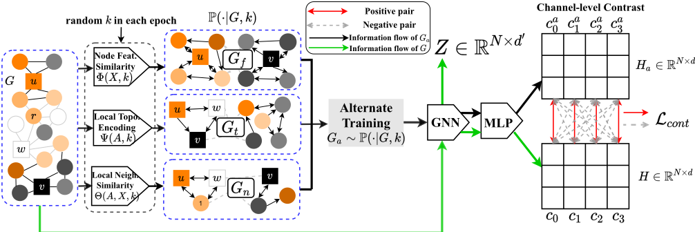
Proximity Graph We reconstruct the graph in both feature and topology spaces to generate augmented views. As shown in Figure 1, the augmentation pool P(·|G, k) consists of three view generators, i.e., Φ(X, k), Ψ(A, k) and Θ(A,X, k). In the feature space, Φ(X, k) aims to build a self-feature proximity graph (FPG) where each node only links to the k nodes with most similar feature vectors, denoted Gf = (Af ,X). Θ(A,X, k) aims to generate a neighborhood feature proximity graph (NPG), where each node links to k most similar nodes in terms of attribute distribution of the feature sets of neighborhoods, denoted Gn = (An,X). In the topology space, Ψ(A, k) builds a topology proximity graph (TPG) where each node links to the top k nodes with most similar local topology, denoted Gt = (At,X). As such, Gf , Gt and Gn are three views of the input graph G. Note that the similarity ranking may be asymmetric so the generated views are directed. In addition, proximity graphs are structural views, therefore the augmentation is only applied to the structure of the graphs rather than the initial node features. Ψ(A, k) means the TPG generator only leverages the structure information A from G, so as other generators.
4 Views Generation
In this section, the instantiation of the generators Φ(X, k), Ψ(A, k) and Θ(A, X, k), is presented.
4.1 Instantiation of Ψ(A, k) for TPG
Figure 1 shows an example where nodes u, v and w have similar local topology: they all have degrees 4, and are connected to 2 triangles, therefore they should be connected in the topology space to construct TPG Gt. To this end, we first encode the structural roles of each node as a vector in the topology space. Although several structural role embedding methods [Ribeiro et al., 2017; Henderson et al., 2012] can do the job, they require separate back-propagation or enumeration operations, which are too heavy as a preprocessing step. Here, we give an alternative method based on graph kernel.
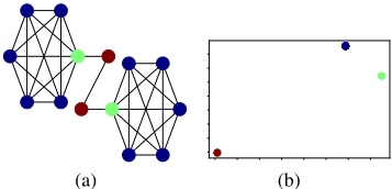
We first extract local subgraphs for all nodes, where the subgraphs can be r-hop egonets (i.e., the induced subgraph surrounding each node) or induced by a set of random walk (RW) sequences starting from each node. We have found that different choices do not affect the results significantly, except that RW which we use here is more efficient for dense graphs. Let S = {S1, · · · , SN} be the set of extracted local subgraphs for each node, we adopt the Weisfeiler-Lehman (WL) subtree kernel [Shervashidze et al., 2011] on the subgraph set S. Then, we can obtain a symmetric positive semi-definite kernel matrix K ∈ RN×N , where Kij denotes the similarity between local subgraphs Si and Sj , which can be seen as the local topological similarity between vi and vj. Then, we can directly factorize K to obtain a low-dimensional representation of each subgraph Si, and this vector is the local topological representation of vi. However, matrix factorization leads to a high computational complexity of O(N 3 ). To solve this problem, we use Nystr¨om approximation [Nikolentzos et al., 2018] to reduce the cost to O(m2N), where m ≪ N. The Nystr¨om method only uses a small subset of m columns of K, such that K ≈ RR⊤ where R ∈ RN×m. Finally, each row of R represents the coordinate of the corresponding node in the graph's topology space, and therefore serves as the local topology representation of the node. Figure 2 shows an experiment on a barbell graph B(6, 2). Based on R, we construct a directed graph where each node links to top-k most similar nodes using outgoing edges, denoted Gt = (At,X). Note that R is only used to generate the structure At of Gt, and node features are still X.
4.2 Instantiation of Φ(X, k) for FPG
Φ(X, k) is defined in the feature space. It generates a selffeature proximity graph (FPG) Gf = (Af , X) directly based on node features X, where each node only links to the k most similar nodes in terms of node features. Figure 1 shows nodes with similar colors (features) are connected to build Gf .
4.3 Instantiation of Θ(A,X, k) for NPG
To capture more complex graph properties which rely on both local topology and node features, we introduce the concept of neighborhood feature proximity graph (NPG): the existence of an edge between two nodes is based on the similarity of their local neighborhoods' features. The rationale behind our idea is that FPG only considers the relationship between individual node features, which is not robust to feature noise. Moreover, in some graphs such as disassortative graphs, harnessing neighborhoods' features while ignoring the self-features can significantly improve the discriminative power of the learned representations [Ma et al., 2021].
Although MPNN-based GNNs obtain a node representation that encodes a rooted subtree around the center node by iteratively aggregating neighborhoods, such a representation does not well reflect the characteristics of a node's neighbors, since it is a mixture of neighbors' features without considering the distribution of each attribute. Hence, Θ measures the similarity between nodes by the distance between the attribute distributions of the feature sets of the nodes' neighborhoods. Given every node's neighborhoods ˆ S = {ˆ Si}Ni=1 , where ˆ Si = Si/ vi is the neighbor set of vi excluding itself. From each ˆ Si, we sample m′ nodes uniformly with replacement to generate a neighborhood feature matrix Xi ∈ Rm′×F for vi, where the k-th attribute is Xi:,k . Then we assume the attribute is a discrete random variable whose realizations depend on the specific pair-wise nodes. Specifically, for vi and vj, the realizations of the k-th attribute are a set of all different values that appear in Xi:,k and Xj:,k , denoted as ωk. We denote the set of all different values in Xi:,k as ωik , then ωik ∪ ωjk = ωk where |ωik |, |ωjk | ≤ m′ . We can vectorize the attribute distribution of Xi:,k as an |ωik |-dimensional vector πik , where πik (t) is the frequency of an attribute value ωik (t) occurs in Xi:,k , and ∑t πik (t) = ∑t πjk (t) = m′ . Then, we measure the neighborhood feature similarity between vi and vj with Wasserstein distance (WD) between the corresponding attribute distributions as D(vi, vj) = ∑Fk=1 W k (vi, vj), where:
where T ∈ R|ωik |×|ωjk | is a flow matrix. In this way, the smaller value of D(vi, vj) indicates the higher similarity between the attribute distributions of the feature sets of two nodes' neighborhoods. As shown in Figure 1, u, w and r have similar neighborhood feature distributions (3 orange and 1 grey), so they are more likely to be connected. Based on the distance measure D(vi, vj), the generator Θ links top-k most similar nodes for each node to build a neighborhood feature proximity graph (NPG) as an augmented view, denoted as Gn = (An,X). Eq. (1) fits the form of WD, which has been well-studied and fast specialized algorithms [Pele and Werman, 2009] have been proposed to solve it.
Summary. FPG and TPG are kNN graphs that use cosine distance to measure node feature similarity and structural similarity, while NPG is a kNN graph based on Wasserstein distance, as we are interested in distribution similarity instead of vector similarity of neighborhoods. These three views are reconstructions of the original graph structure to preserve the high-order interactions between nodes with respect to selffeatures, local topology and distributions of neighborhoods. Now we decide the augmentation pool as P(·|G, k): feeding G and an integer k into the pool, it outputs a view from one of the generators. In the views generation stage, the computational cost mainly comes from calculating the vector similarity for the kNN graphs, which is O(N 2 ). Fortunately, fast approximation and parallelization methods have been well studied to construct kNN graphs efficiently. We are able to construct kNN graphs with local sensitive hashing [Zhang et al., 2013] in O(ln(F + logN)).
5 Proximity Enhanced GCL
We describe each component of PE-GCL in order as depicted in Figure 1.
(1) Alternate training strategy. In each training epoch, we randomly set a k and generate a view Ga ∼ P(·|G, k), where the generator is alternately set to Φ, Ψ or Θ. In other words, each training epoch involves only one augmented view Ga, which is taken turns to set to FPG (Gf ), TPG (Gt) or NPG (Gn). In this way, multiple types of proximity information can be preserved. As compared to joint training with three kinds of views in one epoch, the alternate training strategy reduces computational cost and accelerates the training process. Moreover, the randomness of k helps improve the diversity of views, so that proximity at different scales can be preserved. This also helps to achieve a trade-off among different types of proximity measures. However, repeatedly constructing kNN graphs in each training step is expensive. To address this issue, we limit k to a maximum value kmax, i.e., k ≤ kmax. We only need to find top-kmax neighbors for each proximity graph before training, which is a single-time effort. Then in each training step, an FPG, NPG or TPG with k can be easily obtained from the preprocessed kmax neighbors by masking a certain number of neighbors at the end of the similarity ranking. In practice, kmax is a hyperparameter and kmax < 10 is found to work well.
(2) Shared GNN encoder and projection head. The view Ga ∼ P(·|G, k) together with G are fed into a shared GNN encoder, where each node aggregates the messages propagated from its in-neighbors. We use GAT as the encoder; other MPNN-based GNNs can also be used without much difference in performance. Following the GNN encoder, we use a shared MLP g(·) as a projection head [You et al., 2020] to enhance the expressive power of the output representations. All trainable parameters are shared between two graphs during training.
(3) Channel-level contrastive objective. Unlike most previous methods that construct contrastive pairs between augmented views, PE-GCL constructs contrastive pairs between the original graph and a view. Specifically, the shared MLP outputs two representation matrices H,Ha ∈ RN×d for G and its augmented view Ga respectively, which can be seen as two signals with d channels on two graphs. Some works [Zhu et al., 2020b; Zhu et al., 2020a] focuses on node-level contrasting, which suffers from high computation cost. We offer an alternative method that generates contrastive pairs at the channel level. As shown in the right part of Figure 1, the i-th channels of two output signals, denoted ci and cai , are the ith columns of H and Ha, respectively. Then the contrastive objective aims to maximize the consistency between two representation matrices, such that the same channels ci and cai as inter-graph positive pairs (red solid double-headed arrows) are to be pulled together, and different channels ci and caj,j̸=i as negative pairs (gray dashed double-headed arrow) to be pushed away. Hence, the loss function of pair-wise channels (ci, cai ) is defined as:
| Cora | CiteSeer | PubMed | WikiCS | ACM | CoauthorCS | Texas | Chameleon | Actor | |
|---|---|---|---|---|---|---|---|---|---|
| |V | | 2,708 | 3,327 | 19,717 | 11,701 | 3,025 | 18,333 | 183 | 2,277 | 7,600 |
| |E| | 5,429 | 4,732 | 44,338 | 216,123 | 13,128 | 81,894 | 295 | 31,421 | 26,752 |
| F | 1,433 | 3,703 | 500 | 300 | 1,870 | 6,805 | 1,703 | 2,325 | 932 |
| Classes | 7 | 6 | 3 | 10 | 3 | 15 | 5 | 5 | 5 |
| Input | Type | Algo. | Cora | CiteSeer | PubMed | WikiCS | ACM | CoauthorCS |
|---|---|---|---|---|---|---|---|---|
| A | RW | DeepWalk | 74.49(±0.3) | 49.29(±1.2) | 80.25(±0.3) | 68.33(±1.2) | 60.09(±0.2) 61.15(±0.8) | 85.00(±0.4) 84.97(±0.4) |
| node2vec | 75.72(±0.3) | 51.33(±1.4) | 79.88(±0.2) | 69.06(±0.8) | ||||
| AE | GAE | 81.37(±1.1) | 68.42(±0.6) | 80.81(±0.4) | 68.72(±0.5) | 87.62(±0.7) | 92.46(±0.2) | |
| VGAE | 80.80(±1.3) | 69.60(±0.6) | 82.25(±0.3) | 75.64(±0.6) | 89.78(±0.5) | 92.10(±0.2) | ||
| CL | MVGRL | 83.77(±0.7) | 73.35(±0.5) | 85.33(±0.2) | 74.13(±0.6) | 90.80(±0.3) | 92.08(±0.5) | |
| Unsup | DGI | 83.61(±0.7) | 70.24(±1.4) | 85.31(±0.2) | 75.70(±0.5) | 90.01(±0.3) | 92.30(±0.2) | |
| A,X | 83.24(±0.8) | 71.50(±0.8) | 86.07(±0.2) | 78.26(±0.2) | 90.28(±0.5) | 92.42(±0.2) | ||
| GRACE GMI | 83.51(±0.7) | 72.18(±0.4) | 82.97(±1.0) | 77.57(±0.5) | 87.15(±0.5) | 91.92(±0.1) | ||
| GarphCL | 82.42(±1.2) | 70.80(±0.6) | 78.24(±1.6) | 77.10(±0.3) | 85.03(±0.9) | 86.57(±0.1) | ||
| PE-GCL | 84.12(±0.6) | 72.79(±1.3) | 86.31(±0.6) | 80.33(±1.0) | 91.73(±0.2) | 93.58(±0.0) | ||
| A,X,Y | GNN | GCN | 82.57(±0.2) | 71.81(±0.7) | 86.12(±0.2) | 76.40(±1.0) | 87.66(±1.2) | 93.05(±0.3) |
| GAT | 83.38(±0.2) | 72.50(±0.7) | 84.70(±0.0) | 77.60(±0.6) | 86.52(±1.0) | 92.42(±0.3) | ||
| AM-GCN | 81.15(±0.1) | 74.08(±0.3) | 80.93(±0.2) | 75.92(±0.3) | 91.42(±1.0) | 92.00(±0.1) | ||
| DMGI | 81.73(±0.3) | 71.88(±0.7) | 85.22(±0.1) | 77.42(±0.3) | 89.15(±0.9) | 91.47(±0.2) |
where τ is the temperature hyper-parameter to scale the cosine similarity ϕ(·, ·). [Chen et al., 2020] finds that an appropriate τ can help the model learn from hard negatives. Considering all d channels, the total contrastive loss function is:
Prediction. The GNN encoder and MLP are all trained in an unsupervised manner. After the training stage, the original graph G is fed into the GNN encoder to generate the resulting node embeddings Z, as shown in Figure 1. Then we can apply Z to downstream prediction. See Appendix A for a description of the algorithm.
5.1 Theoretical Analysis
We create three graphs Gf , Gt and Gn as augmented views of G, and then maximize the agreement between the output embedding matrices of G and a view. By this means, the GNN encoder is able to capture richer semantic information (i.e., self-feature similarity, neighborhood feature similarity and structural equivalence), which may boost the subsequent prediction tasks. In other words, minimizing the contrastive
objective in Eq. (3) aims to maximize the "correlation" between the input graph G and its proximity graph Gf , Gt or Gn. However, what does "correlation" precisely mean? In the following, we theoretically discuss the connection between the loss function of PE-GCL and InfoNCE [Kong et al., 2019] to answer this question, and prove that minimizing our proposed channel-level contrastive objective can be viewed as a kind of maximizing a lower bound of the Mutual Information (MI) between G and its views.
Let fθ(c, ca ) = ϕ(g(GNN(G)), g(GNN(Ga)))/τ be the contrastive loss of a specific pair-wise channels c and ca , where θ is parametrized by τ, the GNN encoder GNN(·) and the MLP g(·), we can arrive at the following theorem.
Theorem 1. The contrastive loss in Eq. (3) can be transformed to the InfoNCE form and lower bounded by the MI between H and Ha as:
The proof is in Appendix B. Thus, minimizing Lcont is equivalent to maximizing a lower bound of MI between H and Ha.
6 Experiments and Analysis
6.1 Datasets, Evaluation and Baselines
Datasets. We conduct node classification experiments on the following commonly used six assortative graphs (Cora, CiteSeer, PubMed, WikiCS, ACM and CoauthorCS) [Kipf and Welling, 2017; Mernyei and Cangea, 2020; Sinha et al., 2015]
| Algo. | Texas | Chameleon | Actor |
|---|---|---|---|
| DeepWalk node2vec GAE VGAE MVGRL DGI GRACE | 35.47(±7.6) 31.04(±5.7) 56.22(±4.3) 54.86(±6.1) 63.84(±4.0) 57.03(±6.9) 56.76(±4.8) | 41.16(±6.1) 36.39(±8.2) 48.62(±1.8) 49.26(±1.4) | 26.80(±1.3) 25.78(±1.0) 27.04(±1.2) 27.35(±0.9) 30.52(±0.7) 26.80(±0.8) |
| 55.37(±1.3) | |||
| 51.68(±2.8) | |||
| 53.65(±1.2) | 27.06(±1.2) | ||
| GMI | 53.24(±7.7) | 49.72(±0.8) | 29.51(±0.8) |
| GraphCL | 55.78(±8.2) | 58.35(±1.1) | 28.47(±0.9) |
| PE-GCL | 77.62(±4.9) | 67.66(±1.0) | 36.10(±0.7) |
| GCN | 61.33(±7.7) | 63.96(±1.5) | 30.28(±0.7) |
| GAT | 58.93(±4.3) | 59.21(±0.7) | 26.30(±1.3) |
| AM-GCN | 68.43(±7.4) | 59.77(±2.8) | 29.56(±0.9) |
| DMGI | 57.25(±8.2) | 55.43(±1.9) | 27.57(±0.5) |
and three disassortative graphs (Texas, Chameleon and Actor) [Pei et al., 2019]. The statistics of datasets are in Table 1.
Evaluation Protocol. For assortative graphs, we use ten splits of the nodes into 10%/10%/80% for train/validation/test nodes over 10 random seeds, and run 10 times for each split to report average accuracy with standard deviation. For disassortative graphs, we use the same setting as [Pei et al., 2019]. The model is firstly trained in an unsupervised manner. In the test stage, the original graph is directly fed into the GNN encoder and output a node representation matrix Z ∈ RN×d′ , then the embeddings of the training set are used to train an ℓ2-regularized logistic regression classifier and give the results of classification on the test nodes.
Baselines. PE-GCL 1 is compared with three categories of unsupervised methods: (1) Random walk based methods, including DeepWalk [Perozzi et al., 2014], node2vec [Grover and Leskovec, 2016]. (2) Auto-encoder (AE) based methods, including GAE and VGAE [Kipf and Welling, 2016]. (3) Contrastive learning (CL) based methods, including MVGRL [Hassani and Khasahmadi, 2020], DGI [Veliˇckovi´c et al., 2019], GRACE [Zhu et al., 2020a], GMI [Peng et al., 2020], GraphCL [You et al., 2020]. We also compare PE-GCL with semi-supervised GNNs, including GCN [Kipf and Welling, 2017], GAT [Veliˇckovi´c et al., 2018], AMGCN [Wang et al., 2020], and DMGI [Park et al., 2020].
6.2 Results and Analysis
Overall performance. From Table 2 we can make several observations. (1) Our PE-GCL achieves the best results on five out of the six datasets. Only on CiteSeer dataset, PEGCL is slightly weaker than MVGRL. Considering that MVGRL needs 4 GNN encoders at the same time per epoch, this method suffers from high parameter complexity. By contrast, every component is shared across graphs in PEGCL, so only a single GNN encoder is needed. (2) Although without labels to guide training, PE-GCL still outperforms most semi-supervised methods on most datasets. (3)
1 The source code, hyper-parameter settings and complexity analysis are available at https://github.com/JhuoW/PE-GCL
| Algo. | Cora | Texas | Chameleon |
|---|---|---|---|
| PE-GCL | 84.12(±0.6) | 77.62(±4.9) | 67.66(±1.0) |
| PE-GCL w/o FPG | 83.03(±0.8) | 66.50(±6.5) | 67.53(±0.9) |
| PE-GCL w/o TPG | 84.02(±0.5) | 71.33(±4.7) | 66.57(±1.0) |
| PE-GCL w/o NPG | 82.95(±0.5) | 77.73(±5.8) | 64.42(±2.2) |
GRACE and GraphCL both construct augmented views by imposing random perturbations on the graph, and MVGRL constructs views with diffusion. These methods and our PEGCL achieve comparable or even better results than semisupervised methods. It shows the superiority of CL models on graph learning tasks. (4) Traditional network embedding methods like DeepWalk and node2vec with negative sampling can also be seen as a kind of CL-based method, yet they do not perform well, because node features are ignored, and the number of negative samples is usually very small.
Table 3 shows that PE-GCL consistently yields the best performance on disassortative graphs, where most connected nodes belong to different classes. It demonstrates that our augmented views can help the model capture long-distance correlations between nodes.
Gain fromviews. We propose FPG, TPG and NPG as augmented views to help representations integrate high-order similarity information. However, it is not intuitive howmuch gain is generated by each type of view. To answer this question, we introduce three PE-GCL variants, each of which has one type of view removed. We choose Cora, Texas and Chameleon to conduct the ablation experiments. The results are shown in Table 4. We see that considering FPT and NPG can improve the model accuracy by 1.09%, 1.17% on Cora, while the gain from TPG is small. For Texas, FPG and TPG is important, while NPG may bring about some negative effects. However, for Chameleon, NPG plays a non-negligible role. Thus, our PE-GCL combines these proximity graphs that help achieve balanced gains for general graphs.
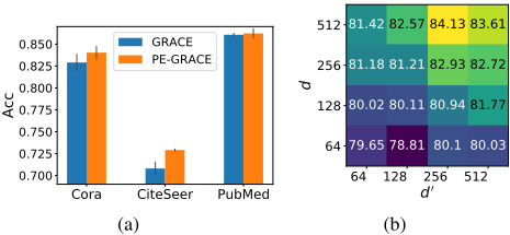
Transferrability. We also show that our proposed three types of views and alternate training strategy can be transferred to other CL-based GNNs. For example, we replace the graph augmentation scheme of GRACE which uses random corruption with proximity graphs, and adopt alternate training strategy, called PE-GRACE. The objective function is still NT-xent [Zhu et al., 2020a] used in the original GRACE. We compare the accuracy of GRACE and PE-GRACE to verify the proximity graphs' adaptability, see Figure 3(a). The results show that proximity graphs can also benefit GRACE and perform better than using random corruption.
| Algo. | Cora | CiteSeer | ||
|---|---|---|---|---|
| AUC | AP | AUC | AP | |
| GAE | 91.37 | 91.99 | 89.53 | 92.02 |
| VGAE | 92.08 | 92.60 | 90.68 | 92.17 |
| GRACE | 91.37 | 92.07 | 92.51 | 92.96 |
| DGI | 91.19 | 91.46 | 90.36 | 90.16 |
| GCN | 91.52 | 91.56 | 90.00 | 90.90 |
| PE-GCL | 92.68 | 93.78 | 95.09 | 94.95 |
Sensitivity analysis. Figure 3(b) shows the impact of hidden layer sizes of the GNN encoder and the MLP on the classification results of PE-GCL on Cora. With the increase of dimensionalities, the performance increases first and starts to stabilize when the dimensionalities reaches 256.
6.3 Link Prediction
For link prediction, we conduct experiments on Cora and CiteSeer, removing 5% existing edges and the same-size nonexisting edges for validation, 10% existing edges and the same-size non-existing edges for testing. We compute the predicted adjacency matrix by Apred = Sigmoid(ZZ ⊤) and report the AUC and AP in Table 5. The PE-GCL achieve the highest prediction scores among baselines indicating that PE-GCL has better reasoning ability for network connectivity and can better retain similarity information between nodes.
7 Conclusion
In this work, we propose PE-GCL, a self-supervised representation learning framework based on contrastive learning. PE-GCL aims to preserve multiple types of proximity information based on different definitions of node similarity. In PE-GCL, we propose proximity-based graph views based on self-feature similarity, local topology similarity and neighborhood feature similarity. Then we use a contrastive objective to maximize the agreement of the views and the original graph. In particular, we construct contrastive pairs on a channel level, by which we can greatly reduce the number of negative pairs. Experimental results show that PE-GCL is competitive against state-of-the-art methods.
A The Pseudocode of PE-GCL
The details of PE-GCL are described in Algorithm 1.
B Proof of Theorem 1
Proof. Given two view sets A and B, both with the same cardinality n, there exists a bijection π : A → B such that each view of one set is positively paired with exactly one view of the other set. Any other inter-set pairs are negative. Under
Algorithm 1 PE-GCL
- 1: Input: GraphG = (V,E,X); Upper limit of the number of neighbors kmax; Number of iterations T ; Temperature hyper-parameter τ; Dimension of the projection head d; Dimension of the GNN encoder d′
- 2: ̂ Af ← Φ(X, kmax); ̂ At ← Ψ(A, kmax); ̂ An ← Θ(A, X, kmax)
- 3: for t = 1, 2, · · · , T do
- 4: Random sample k ≤ kmax
- 5: Ω = Alternately sample a generator from {Φ,Ψ,Θ}
- 6: Aa =Mask(Ω(A, kmax), kmax -k) ▷ Mask the kmax - k least similar neighbors for each node
- 7: Ga = (Aa,X)
- 8: Z ←GNN(G), Za ←GNN(Ga)
- 9: H ← g(Z), Ha ← g(Za)
- 10: Lcont ←Eq.(3)
- 11: end for
this condition, InfoNCE which is upper bounded by MI, can be defined as:
where Q = ((a1, b1), · · · , (an, bn)), in which each pair as an element in Q represents a positive pair, fθ(·) ∈ R is a function parameterized by θ, P(Q) is the distribution of positive pairs, which is uniform. Then our contrastive objective Eq. (3) can be rewritten as the expectation form:
where Ha = g(GNN(Ga)), dimension d is a constant. To fit Eq. (4), we set A = H, B = Ha, then (ci, cai ) is a realization of the random variable Q. Here we consider H and Ha as two view sets, and each column of H and Ha, i.e., ci and cai are regarded as the views they are in. Thus, Q = ((c1, cai ), · · · , (cN, caN )), where (ci, cai ) is a positive pair. ci and caj form a negative pair, where i ̸= j. Hence, P(ci, cai ) = P(Q) is a discrete uniform distribution of size d, so P(ci, cai ) = P(cai ) = P(ci). Let fθ(c, ca ) = ϕ(g(GNN(G)), g(GNN(Ga)))/τ, where θ parametrized by τ, the GNN encoder and the MLP g(·). Then Eq. (5) can be transform to the InfoNCE form in Eq. (4) as:
here we omit the constant 2 log d, which concludes the proof.
Acknowledgements
This work is supported in part by Shenzhen Baisc Research Fund under grant JCYJ20200109142217397.
@inproceedings{ijcai2022p340,
  title     = {Proximity Enhanced Graph Neural Networks with Channel Contrast},
  author    = {Zhuo, Wei and Tan, Guang},
  booktitle = {Proceedings of the Thirty-First International Joint Conference on
               Artificial Intelligence, {IJCAI-22}},
  publisher = {International Joint Conferences on Artificial Intelligence Organization},
  editor    = {Luc De Raedt},
  pages     = {2448--2455},
  year      = {2022},
  month     = {7},
  note      = {Main Track},
  doi       = {10.24963/ijcai.2022/340},
  url       = {https://doi.org/10.24963/ijcai.2022/340},
}
TY - CPAPER TI - Proximity Enhanced Graph Neural Networks with Channel Contrast AU - Zhuo, Wei AU - Tan, Guang T2 - Proceedings of the Thirty-First International Joint Conference on Artificial Intelligence, IJCAI-22 PB - International Joint Conferences on Artificial Intelligence Organization PY - 2022 SP - 2448 EP - 2455 DO - 10.24963/ijcai.2022/340 UR - https://doi.org/10.24963/ijcai.2022/340 ER -Copied
Machine-readable versions of this paper, for tools and AI agents:





