Beyond Strong-Cyclic: Doing Your Best in Stochastic Environments

1 Introduction

Planning in nondeterministic environments is one of the key challenges of AI: often the agent does not have control over everything that happens in its environment so it views the environment as nondeterministic (in a devilish sense), i.e., only partially controllable by the agent itself. This topic has developed as a subarea of Planning on Fully Observable Nondeterministic Domains (FOND) [Rintanen, 2004; Geffner and Bonet, 2013; Ghallab et al., 2016; Haslum et al., 2019] and numerous solvers are available [Mattm¨uller et al., 2010; Kissmann and Edelkamp, 2011; Muise et al., 2012; Ram´ırez and Sardi˜na, 2014; Geffner and Geffner, 2018].

The direct extension of classical planning to FOND gives rise to strong plans, i.e., policies or strategies that tell the agent what to do in every situation and that achieve the goal in spite of the nondeterministic environment's response to the agent's actions [Cimatti et al., 1998; Pistore and Traverso, 2001]. However, in many situations these kinds of plans do not exist. So, a weaker notion of plan was introduced, the strong cyclic plans [Daniele et al., 1999; Cimatti et al., 2003]. Intuitively, these policies allow loops from which the agent assumes it will eventually exit, e.g., they may encode trial-and-error strategies. Interestingly, as recently noted in [D'Ippolito et al., 2018], the fundamental question of formalizing "contexts under which these type[s] of plans will indeed achieve the objectives. . . has not received much attention and has mostly been discussed informally". A first attempt to characterize these contexts has been to make a logical fairness assumption on the actions effects, see [D'Ippolito et al., 2018] for a discussion. Unfortunately, while this solves the problem for classical reachability goals, if we consider temporally extended goals, e.g., expressed in LTL or LTLf , this characterization fails because the simple fairness assumption that is sufficient for reachability is not adequate for LTL or LTLf goals [Aminof et al., 2020b]. An alternative to logical fairness is stochastic fairness (see [Aminof et al., 2020b] for a detailed comparison) already suggested in early papers, e.g., [Cimatti et al., 2003]. This point of view assumes that the nondeterminism in FOND arises from a stochastic nature of the environment: the environment is not adversarial to the agent, but chooses its effects according to some unknown probability distribution. In particular, strong-cyclic policies rely on the fact that in a stochastic environment, repeating an action (in the same situation) will eventually lead to the desired effect.

The question now arises: on what objects is this unknown probability distribution given? Is it given on the current values of the fluents and the action, and if so, what is the justification for that? Why should we assume such a probability distribution is stationary with respect the domain states? After all, the nondeterministic domain describes only the support, i.e., the effects with non-zero probability. No further assumptions should be made on the effect distributions. In this paper we take this observation seriously.

We focus on stochastic domains and LTL and LTLf goals. We study three classes of policies: (i) those that almostsurely enforce the goal, i.e., with probability 1, [Baier et al., 2008], (ii) those that are optimal wrt enforcing the goal [Puterman, 2005], and (iii) those that are best-effort wrt enforcing the goal [Aminof et al., 2021b]. The latter, which we call stochastic best-effort policies, are novel in the context of stochastic domains. Such a policy will guarantee that even if the goal is not achievable with probability 1, it will, intuitively, seize every opportunity to achieve the goal. For example, suppose an agent is offered some money that, if it were to accept, can only be used to place one of two bets, Bet 1 or Bet 2, each of which gives it a non-trivial probability of winning; however, the agent does not know these probabilities, or even which probability is larger. If the agent's goal is to win money at the casino, what actions should it take? In this setting the agent cannot guarantee with probability 1 that it will win a bet. Also, since the relative probabilities of winning each bet are not known, it can't deduce an optimal policy either. A rational solution would be to accept the money, rather than refuse the money, and place either bet. This is achieved by a stochastic best-effort policy.

In Section 3, we show the following: optimal policies are stochastic best-effort, but a stochastic best-effort policy need not be optimal; if an almost-sure policy exists, the stochastic best-effort policies are exactly the almost-sure policies; stochastic best-effort policies always exist, while almost-sure or optimal policies may not exist.

In Section 4, we consider a FOND as a specification of a set of stochastic domains, i.e., those whose support is specified by the FOND. We show that a finite-state policy that is stochastic best-effort in one of these stochastic domains is in fact stochastic best-effort in all of these stochastic domains. This immediately provides an algorithm to compute a single stochastic best-effort policy that works for each of the stochastic domains induced by the FOND: choose a stochastic domain compliant with the FOND in the most convenient way (e.g., assigning uniform probability to all nondeterministic transition of the FOND), and compute a (finite-state) optimal policy for that particular stochastic domain. Note that the stochastic domain can be chosen to be an MDP, which always has an optimal policy. This policy is in fact stochastic besteffort for every stochastic domain specified by the FOND. Moreover, if the policy almost-surely enforces the goal in that stochastic domain then it almost-surely enforces the goal in every stochastic domain specified by the FOND.

In other words, we show that the true nature of FOND for strong cyclic-plans (or FOND under "stochastic fairness") is that of a generalized planning problem [Srivastava, 2010; Bonet et al., 2010; Hu and De Giacomo, 2011; Bonet et al., 2017] over the set of stochastic domains induced by the FOND. Moreover, our studies show that even if the strong cyclic solution does not exist, instead of giving up, we can provide a best-effort solution anyway, which unlike optimal solutions is robust in that it is shared by all induced stochastic domains. Observe that this last aspect is of interest per se since it can also be understood as follows: even if the probabilities in a stochastic domain, such as an MDP, are not accurate for some reason, as long as the support is correct, the nominal optimal solution, although not optimal in reality remains best-effort anyway.

2 Preliminaries

Notation

Sequences may be written (x0, x1, · · · ) or x0x1 · · · . If h is a finite sequence then last(h) is its last element. If h is a prefix of h′ we say that h′ extends h. A set is countable if it is finite or countably infinite. Let Dbn(X) denote the set of distributions over X, i.e., functions d : X → [0, 1] such that ∑x∈X d(x) = 1. An element x is in the support of d if d(x) > 0.

Stochastic Domains

Let F be a finite set of Boolean variables called fluents. We write Obs = 2F for the set of evaluations of the fluents, sometimes called observations or percepts. For symmetry, let A be a finite set of Boolean variables (disjoint from F) and let Act = 2A be the set of actions. A stochastic domain D is a tuple (F, A, s0, Pr) where

1. s0 ∈ Obs is the initial observation, and
2. Pr : Hist ×Act → Dbn(Obs) is the transition function. Here Hist is the set of histories, i.e., sequences (s0, a0, s1, a1, · · · , sk) that start with the initial observation, alternate observations and actions, and end in an observation.

The support function of D is the function ∆ : Hist ×Act → 2Obs defined by s ∈ ∆(h, a) iff Pr(h, a)(s) > 0. If Pr(h, a)(s) > 0 we say that s is in the support of Pr(h, a). We say that D has Markovian support if ∆(h, a) only depends on last(h) and a, i.e., last(h) = last(h′ ) implies that ∆(h, a) = ∆(h′ , a). In this case, we may write the support function as ∆ : Obs × Act → 2Obs . We say that D is bounded if there is some ϵ > 0 such that Pr(h, a)(s) ≥ ϵ for all h, a and s in the support of Pr(h, a). A domain is Markovian if Pr(h, a) only depends on last(h) and a, i.e., last(h) = last(h′ ) implies that Pr(h, a) = Pr(h′ , a).

Note that finite-state Markov Decision Processes (MDPs) without rewards are exactly the Markovian stochastic domains. Some of the counterexample stochastic-domains that we give are MDPs; in the figures, we will label their transitions by a : r to mean that, given that action a was played, the probability of that transition is r.

Plays and Policies

Let D = (F,A, s0, Pr) be a stochastic domain. A play of D is an infinite sequence π = (s0, a0, s1, a1, · · · ) starting in the initial observation. Let Plays denote the set of all plays in D. A policy (aka strategy, plan) is a function σ : Hist → Act. A σ-play (resp. σ-history) is such that σ(s0, a0, s1, a1, · · · , st) = at for every t. A policy is finitestate if it can be represented as a finite-state input/output automaton that, on reading h ∈ Hist as input, outputs the action σ(h). A policy is memoryless if last(h) = last(h′ ) implies that σ(h) = σ(h′ ). In this case we can write σ : Obs → Act.

Markov Chains

A Markov chain M is a tuple (Q, s0, p) where Q is a countable set of states, s0 ∈ Q is the initial state, and p : Q → Dbn(Q). We write p(s, t) for p(s)(t), and call these the transition probabilities of M. The graph (Q, EM) induced by M

has state set Q and edge set EM consisting of pairs (q, q′ ) such that q′ is in the support of p(q). Thus, graph-theoretic notions (like connected components) are defined for M by considering the induced graph. A Markov chain is finite if Q is finite. A Markov chain M induces a canonical probability space on the set of infinite paths in M starting in s0 that we denote (ΩM,AlgM, µM), e.g., [Puterman, 2005]. We may drop subscripts for readability. Elements of Alg are called events. All sets that we measure are either assumed to be events, or can be shown to be events, although we may not explicitly say so. For a history h we denote by Ch the event consisting of the plays with prefix h. If µ(E) = 1 we say that almost surely E holds (in M). In case µ(F) > 0 define µ(E|F) := µ(E ∩F)/µ(F).

Probability Measures

Fix a domain D and a policy σ. Define the Markov chain D[σ] = (Hist, s0, p) where p(h, h′ ) := Pr(h, σ(h))(s) for h′ = hσ(h)s. The measure of the induced probability space is denoted µD[σ]. Note that a play in D[σ] is a sequence of histories of D, i.e., of the form (s0), (s0, a0, s1), (s0, a0, s1, a1, s2), · · · , whose limit is a play in D, i.e., of the form (s0, a0, s1, a1, · · · ). Thus, for convenience, we will refer to σ-plays in D as plays in D[σ], and vice versa. Intuitively, µD[σ](E) is the probability that a play in D starting from s0 generated by σ is in E. We say that σ almost surely enforces E (in D) if µD[σ](E) = 1.

Linear-time Temporal Logic (LTL/LTLf)

The formulas of LTL a finite set AP of atoms are defined by the following BNF (where p ∈ AP): ϕ ::= p | ϕ ∨ ϕ | ¬ϕ | Xϕ | ϕUϕ. We use the usual abbreviations, Fϕ .= trueUϕ, Gϕ .= ¬F¬ϕ. A trace τ is an infinite sequence of valuations of the atoms, i.e., τ ∈ (2AP )ω . For n ≥ 0, write τn for the valuation at position n. Given τ, n, and ϕ, the satisfaction relation (τ, n) |= ϕ, stating that ϕ holds at step n of the sequence τ, is defined as follows: 1. (τ, n) |= p iff p ∈ τn; 2. (τ, n) |= ϕ1 ∨ ϕ2 iff (τ, n) |= ϕ1 or (τ, n) |= ϕ2; 3. (τ, n) |= ¬ϕ iff (τ, n) |= ϕ does not hold; 4. (τ, n) |= Xϕ iff (τ, n + 1) |= ϕ; and 5. (τ, n) |= ϕ1 Uϕ2 iff there exists m ≥ n such that: (τ,m) |= ϕ2 and (τ, j) |= ϕ1 for all n ≤ j < m. If τ, 0 |= ψ we write τ |= ψ and say that τ satisfies ψ and that τ is a model of ψ. In case AP = F ∪A, we say that a play (s0, a0, s1, a1, · · · ) satisfies ϕ if the corresponding trace (s0∪a0, s1∪a1, · · · ) satisfies ϕ. We also consider the variant LTLf (Bacchus and Kabanza [2000], Baier and McIlraith [2006], De Giacomo and Vardi [2013]). It has the same syntax and semantics as LTL except that τ is a finite sequence and X and U are redefined as follows: for n < |τ| define τ, n |= Xψ if n < |τ| - 1 and τ, n + 1 |= ψ; define τ, n |= ϕ1 U ϕ2 iff there exists m with n ≤ m < |τ | such that (τ,m) |= ϕ2 and (τ, j) |= ϕ1 for all n ≤ j < m. 1

We use the following convention for interpreting LTLf formulas over infinite traces: if τ is infinite and ψ is an LTLf formula, then τ |= ψ means that some finite prefix of τ satisfies ψ (analogous to the agent using an explicit "stop" action).

1 "Optimistic" variants of these operators can be defined, e.g., "weak next ψ" holds if n < |τ | - 1 implies τ, n + 1 |= ψ.

Goals and Planning Problems

A planning problem (D,G) consists of a stochastic domain D and a set G of plays, called a goal. We say that a play satisfies G if it is in G. We only require that G satisfies the following technical property: for every policy σ, the set of plays of D[σ] that are in G is measurable. This includes goals represented by LTL/LTLf formulas and by automataM. If D is stochastic, we will write µD[σ](G) for the measure of the event consisting of all plays in D[σ] that are in G.

3 Stochastic Best-effort (SBE) Policies

In this section we provide the definition of stochastic besteffort policy, and compare it to optimal policies. Fix a stochastic domain D and a goal G. For a policy σ, and σhistory h, define valD,G(σ, h) (simply val(σ, h)) as follows:

The following fact about the extreme values follows from additivity of µD[σ]:

Proposition 1 (Hereditary). If val(σ, h) ̸= 0, and h′ is σhistory that extends h, then val(σ, h) = val(σ, h′ )

Here is the main definition of this work:

Definition 1 (Stochastic best-effort - SBE). Fix a stochastic domain D and a goal G. A policy σ is called stochastic besteffort (SBE) for the planning problem (D,G) if for every σhistory h of D:

Intuitively, an SBE policy tries, from every history, to almost-surely enforce G, and if this is not possible, then at least tries to ensure that G holds with positive probability. Thus, even if there is no policy that almost-surely enforces G from the start, the coin tosses from the environment may lead to such an opportunity in the future, and an SBE policy will take advantage of this. By maintaining a positive probability where possible, SBE policies do not close the door on opportunities that may arise due to stochasticity. Moreover, differentiating between probability zero, non-zero, and one, turns out to be robust even if very little is known of the probabilities themselves, but only what is and is not possible, see Section 4. It turns out that SBE policies always exist!

The proof of this result is an adaptation of the fact that besteffort policies exist in the context of synthesis under assumptions [Aminof et al., 2020a]. Moreover, the special case of temporal goals and bounded stochastic domains with Markovian support will follow from Theorem 4 Part 1.

3.1 Relation to Optimization Problems

In the case that probabilities in a stochastic domain are known or can be sampled, the natural problem is to find optimal policies, i.e., ones that maximize the probability of success. A policy σ is optimal for the planning problem (D,G) if σ = argsupσ′µD[σ′ ](G). It is interesting to note that, in contrast to SBE policies, optimal policies don't always exist, even for reachability goals:

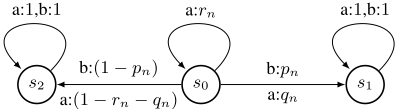
Example 1 (Optimal need not exist). Consider Fig. 1 where pn := (n+1)/(2n+3) and rn := 1 (and thus qn := 0). One can calculate that for every policy σ, µD[σ](G) < 1/2, while supσ µD[σ](G) = 1/2. We remark that D is bounded and has Markovian support.

Optimal policies are stochastic best-effort:

Theorem2 (Optimal→SBE). Let Dbe a stochastic domain, and let G be a goal. Then every optimal policy σ for (D,G) is stochastic-best effort for (D,G).

Proof. Suppose σ is not stochastic best-effort. Then val(σ, h) < val(σ′ , h) for some σ′ and some history h that is both a σ-history and a σ′ -history. There are two cases depending on val(σ, h) ∈ {-1, 0}. We consider the case that val(σ, h) = 0. In this case, µD[σ](G|Ch) = 0 and µD[σ′ ](G|Ch) > 0. Define the policy σ′′ := σ[h ← σ′ ], which agrees with σ′ on h and all of its extensions, and otherwise agrees with σ. Then µD[σ′′ ](G|Ch) > 0, and thus µD[σ′′ ](G) > µD[σ](G). Thus σ is not optimal. The case that val(σ, h) = -1 is similar.

We point out that the converse is false already for reachability goals. Although one can deduce this from the fact that optimal policies don't always exist (Example 1) while SBE policies do (Theorem 1), it also holds for finite MDPs and reachability goals for which optimal policies always exist.

Example 2 (SBE ̸→ optimal). Consider Fig. 1 with pn := 1/10, qn := 7/10, and rn = 0. The domain is an MDP. Only the first action played is relevant; thus there are in effect just two policies "first do a", which is optimal and achieves the goal with probability 7/10, and "first do b", which is not optimal (it achieves the goal with probability 1/10). However, both policies are SBE (since both have value 0 at s0).

By Proposition 1 and Definition 1 we get:

Theorem 3. Let D be a stochastic domain and G a goal. If there is a policy σ that almost-surely enforces G in D, then a policy σ′ is stochastic-best effort for (D,G) if and only σ′ almost-surely enforces G in D.

This has an analogue in the non-stochastic setting: if there is a winning policy, then the best-effort policies are exactly the winning policies [Aminof et al., 2020a].

4 Generalized Stochastic Planning

Finding a single policy that works in multiple "similar" domains is called "Generalized Planning". In this section we introduce and study generalized planning for stochastic domains. We restrict to stochastic domains that are bounded and have Markovian support: the latter means we can talk about an induced nondeterministic domain that does not change over time; the former means this domain does not change "in the limit" (intuitively, if the probability of taking a transition (s, a, s′ ) goes to zero very fast, then the probability conditioned on being at s infinitely often of eventually taking the edge may go to zero, which means, intuitively, that this edge is not there "in the limit").

Definition 2. Let D1,D2 be stochastic domains that are bounded and have Markovian support. We say that D1 and D2 are similar if they have the same set of fluents F, actions A, initial observation s0, same support functions, but possibly different Pr. A generalized planning problem is a pair (D,G) where D is a set of pairwise-similar stochastic domains, and G is a goal for every D ∈ D.

We specify G by LTL/LTLf formulas (and in some proofs also with automata), and we specify D by a fully observable nondeterministic domain (FOND) D = (F, A, s0, ∆), where ∆ : Obs × Act → 2Obs \ {∅}. That is, D determines the set D of bounded stochastic domains D′ = (F, A, s0, Pr) such that ∆ is the support function of Pr.

Definition 3. Let (D,G) be a generalized planning domain. A policy is stochastic best-effort (SBE) (resp. optimal, resp. almost-sure enforcing) if for every domain D ∈ D, the policy is stochastic best-effort (resp. optimal, resp. almost-sure enforcing) for the planning domain (D,G).

It is not hard to see that already in very simple cases there may not be a policy that is optimal for D, even though for every D ∈ D there is an optimal policy.

Example 3. Recall the domain from Example 2 that has an optimal policy. Define a similar domain D′ with the roles of a and b reversed, i.e., pn := 7/10, qn := 1/10, rn := 0. Then the optimal policy in D′ is "first do b". So, there is no policy that is optimal for both (D,G) and (D′ ,G).

On the other hand, as we now show, already in a quite general setting there is a stochastic best-effort policy for (D,G).

Theorem 4. Let (D, ϕ) be a generalized planning problem for a LTL/LTLf goal ϕ. Then:

1. There exists a finite-state SBE policy for (D, ϕ) which can be computed from the specification of D (i.e., the common Markovian support) and ϕ (i.e., the LTL/LTLf formula).
2. If σ is a finite-state SBE policy for (D, ϕ) for some D ∈ D, then σ is a SBE policy for (D, ϕ). Moreover, if σ almost-surely enforces ϕ for some D ∈ D, then σ is almost-surely enforcing for (D, ϕ).

The algorithm for Part 1 is simple. Given the support ∆ : Obs × Act → 2Obs \ {∅} and LTL/LTLf formula ϕ:

• Step 1. Fix a similar finite MDP D = (F,A, s0, Pr) by letting Pr(s, a) be, e.g., the uniform distribution over ∆(s, a): Pr(s, a)(s′ ) := 1/|∆(s, a)| for s′ ∈ ∆(s, a).
• Step 2. Return a finite-state optimal σ for the stochastic planning problem (D, ϕ). This can be computed using any standard technique, e.g., [Bianco and de Alfaro, 1995].

Remark 1. Consider finite nondeterministic domains D = (F,A, s0,∆) and reachability goals Fϕ. An important concept in this context are strong-cyclic policies, e.g., [Cimatti et al., 2003]. A view for such policies is that D abstracts a single finite MDP whose exact probabilities are unknown, but whose support is known, and strong-cyclic policies almostsurely enforce Fϕ. Theorem 4 (Part 2) implies that one can take a much broader view: strong-cyclic planning can be viewed as finding a policy that is almost-sure enforcing for generalized stochastic planning consisting of infinitely many, not-necessarily Markovian, similar stochastic domains.

In the special case of strong-cyclic solutions, it was noted in [Jensen et al., 2001] that one can find such solutions by simply choosing a convenient instantiation and solving it for optimality. Our algorithm (Theorem 4, Part 1) extends this result in three directions: (1) LTL/LTLf instead of just reachability; (2) generalized stochastic planning instead of finite MDPs; (3) SBE instead of simply enforcing almost-surely.

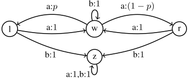
Remark 2. Part 2 fails if we remove any of the three assumptions, i.e., policies being finite-state, domains being bounded, domains having Markovian support: (i) If σ is not assumed finite-state, consider the stochastic domain from Fig. 2. There is a non finite-state policy σ that almost-surely enforces the goal iff p ≤ 1/2. Intuitively, the policy σ simulates a onedimensional random walk on N0 starting at 1, stopping at 0, where p is the probability of decrementing; and uses the fact that the random walk almost-surely stops iff p ≤ 1/2, see, e.g., [Bhattacharya and Waymire, 2021]. The policy σ keeps a counter k ∈ N0 as memory: if k = 0 and observe "l" or "r" then choose action "b", otherwise choose action "a"; decrement (resp. increment) the counter when observing "l" (resp. "r"). (ii) If domains are not assumed to be bounded, consider two domains D,D′ instantiated from Fig. 1 with pn := 0 and rn := 1 - qn. For D let qn := 1/3, and for D′ let qn := 1/3n+1 . Then consider the policy that always plays a. (iii) If the domains are not assumed to have Markovian support, consider D1,D2 instantiated from Fig. 1 with rn := 1. Domain D1 is defined p0 := 1 and pn := 0 for n > 0, while D0 is defined by p0 := 0 and pn := 1 for n > 0. Then consider the policy that immediately plays b.

4.1 Automata-theory Preliminaries

We define the (synchronous) product of a deterministic automaton and a stochastic domain. This allows us to reduce finite-state policies to memoryless policies, and to work with automata acceptance conditions instead of LTL/LTLf goals.

A deterministic automaton is a tuple M = (Σ,Q, q0, δ) where Σ is the input alphabet, Q is a finite set of states, q0 ∈ Q is the initial state and δ : Q×Σ → Q is the transition function. A (finite or infinite) input string u = u0u1 · · · determines a unique run, i.e., the sequence q0q1 · · · of states starting with the initial state such that δ(qi, ui) = qi+1 for all 0 ≤ i < |u|. We use labeling functions λ : Q → L that map the automaton states Q to some set of labels: we set L = Act to model the decisions taken by finite-state policies; we set L = {0, 1} to model reachability objectives for deterministic finite word automata (DFAs); we set L ⊆ Z to model parity objectives for deterministic parity word automata (DPAs). A DFAMaccepts a finite string u if λ(qi) = 1 for the last state qi of the run of M on u. A DPAM accepts an infinite string u if limsupi→∞λ(qi) is even, where the qi are the states of the infinite run of Mon u (i.e., if the largest integer that occurs infinitely often as a label of a state in the run is even).

We now define the product of a deterministic automaton and a stochastic domain. Intuitively, the product will result in a stochastic domain with the "same" distribution, i.e., the product domain D × M mimics the probabilistic choices of D while also deterministically storing the state that M would reach given the history so far. Here is the construction. Let D = (F,A, s0, Pr) be a stochastic domain and let M = (Σ,Q, q0, δ) be a deterministic automaton with Q = 2B for some set B of Boolean variables disjoint from F (this is a technical convenience), and Σ = 2F∪A. Define the synchronous product D ×M to be the stochastic domain (F ∪ B,A, s0 ∪ q0, Pr′ ) where the probability distribution Pr′ is defined as follows. For a history x = (s0 ∪ q0, a0, s1 ∪ q1, a1, · · · , sk ∪ qk) of the product, and a ∈ Act , the support of Pr′ (x, a) is the set valuations s ∪ q such that (i) s is in the support of Pr((s0, a1, s1, a1, · · · , sk), a), and (ii) q = δ(qk, sk ∪ a), and in this case, Pr′ (x, a)(s ∪ q) = Pr((s0, a0, s1, a1, · · · , sk), a). Every labeling function λ : Q → L can be lifted to D ×M by setting λ(s, ℓ) := λ(ℓ).

We note that because we only consider deterministic automata, policies over D and over D ×M are in correspondence, and the measure of events is unchanged by this correspondence. We now state this formally. We say that a history (s0, a0, · · · , sk) in D induces a history (s0 ∪q0, a0, s1 ∪ q1, a1, · · · , sk ∪ qk) in D×M, by adding the corresponding automaton state qi+1 = δ(qi, (si ∪ai)) for every i. Likewise, we say that a policy σ in D induces a policy σ′ in D ×M, and an event E of D[σ] induces an event E′ of (D×M)[σ′ ]. The following is a direct result of the above definitions:

Lemma 1. For a stochastic domainD and an automatonM, consider the product stochastic domain D ×M. Let σ be a policy and let E be an event of D[σ]. Moreover, let σ′ be the induced policy and let E be the induced event of (D×M)[σ′ ]. Then, µD[σ](E) = µ(D×M)[σ′ ](E′ ).

We recall the following fundamental fact of automatatheoretic approaches to reasoning about LTL/LTLf :

Theorem 5. [Vardi and Wolper, 1986] There is an algorithm that takes an LTL (resp. LTLf ) formula ϕ and constructs a DPA (resp. DFA) Mϕ that accepts the models of ϕ.

Lemma 1 and Theorem 5 immediately allow us to reduce problems about planning for LTL/LTLf objectives, to problems about planning for parity/reachability objectives:

Corollary 1. Let D be a stochastic domain, let σ be some policy, let ϕ be an LTL (resp. LTLf ) formula and let Mϕ be the corresponding DPA (resp. DFA) with parity (resp. reachability) objective C. Moreover, let σ′ be the induced policy of D ×Mϕ. Then, µD[σ](ϕ) = µ(D×Mϕ)[σ′ ](C).

4.2 Values Transfer Across Similar Domains

In this section we show how to compare valD1,G(σ, h) and valD2,G(σ, h) for similar domains D1, D2. We begin assuming G is a parity goal and σ is memoryless, and end assuming G is an LTL/LTLf formula and σ is finite-state.

Suppose D is a stochastic domain with Markovian support and let ∆ : Obs × Act → 2Obs be the support function. A play π = (s0, a0, s1, a1, · · · ) in D is called state-action fair if for every triple (s, a, s′ ) with s′ ∈ ∆(s, a), if there are infinitely many i such that si = s and ai = a, then there are infinitely many i such that si = s, ai = a, and si+1 = s′ . The next lemma follows from [Baier and Kwiatkowska, 1998]; intuitively, if a transition has positive probability, then the probabilitity of visiting its source and not taking the transition goes to zero as the number of visits goes to infinity:

Lemma 2 (State-action fair). Let D be a bounded stochastic domain with Markovian support, and σ a policy. Let E be the set of state-action fair plays. Then µD[σ](E) = 1.

For memoryless policies and parity goals, we can relate satisfaction almost-surely to satisfaction on all state-action fair plays. The reason this is possible is that state-action fairness guarantees that every play will eventually reach a bottom strongly-connected component and that every state in this component will be visited infinitely often:

Lemma 3. Let D be a bounded stochastic domain with Markovian support, C : Obs → Z be a parity objective, and σ : Obs → Act be a memoryless policy. Then, µD[σ](C) = 1 iff all state-action fair plays in D[σ] satisfy C.

We can now show that values transfer for parity goals; this follows from Lemma 3 using that parity conditions are closed under complement and that the satisfaction of a parity condition does not depend on finite prefixes:

Theorem 6. Let D1,D2 be similar stochastic domains (that are bounded and have Markovian support). Let h be a history, σ : Obs → Act be a finite-state policy, and C : Obs → Z be a parity objective. Then valD1,C(σ, h) = valD2,C(σ, h) for every σ-history h.

Combining Theorem 6 with Lemma 1 and Corollary 1 we can show that values transfer for LTL/LTLf goals:

Theorem 7. Let D1,D2 be similar stochastic domains. Let ϕ be an LTL/LTLf goal, and let σ be a finite-state policy. For every σ-history h, valD1,ϕ(σ, h) = valD2,ϕ(σ, h).

We are now in a position to finish the proof of Theorem 4. To see that the algorithm in Part 1 is correct, note that by Theorem 2, the finite-state policy σ produced by the algorithm is SBE for (D, ϕ). Since D is bounded, by Theorem 7 also σ is SBE for (D′ , ϕ) for every D′ ∈ D. To see that Part 2 is correct, simply apply the definitions and Theorem 7.

5 RelatedWork

Variants of "best-effort" policies are studied for the nonstochastic setting in Reactive Synthesis [Aminof et al., 2020a; Aminof et al., 2021b; Aminof et al., 2021a] and in games on graphs [Berwanger, 2007; Faella, 2009; Brenguier et al., 2017].

Stochastic domains in this paper are countable and not necessarily Markovian. Memory requirements for ϵ-optimal policies for countable Markovian domains with parity objectives were studied in [Kiefer et al., 2020].

Various traditional notions of plan correctness for generalized planning for infinite stochastic domains with reachability goals are studied in [Belle and Levesque, 2016], which in addition, characterizes the strong-cyclic policies for generalized planning problems specified by a finite-state nondeterministic domain (with varying initial states). In contrast, the generalized planning problem in our work consist of infinitely many stochastic domains in which the probabilities are different.

The finite domain D that specifies the set of similar domains D can be viewed as an abstraction D. This point of view has been exploited to solve (non-stochastic) generalized planning problems in [Bonet et al., 2017; Bonet et al., 2020].

Acknowledgments

Partially supported by the Austrian Science Fund (FWF) P 32021; ERC Advanced Grant WhiteMech (No. 834228); EU ICT-48 2020 project TAILOR (No. 952215); PRIN project RIPER (No. 20203FFYLK); JPMorgan AI Faculty Research Award "Resilience-based Generalized Planning and Strategic Reasoning".