
Plausibility Reasoning via Projected Answer Set Counting - A Hybrid Approach
Proceedings of the Thirty-First International Joint Conference on Artificial Intelligence. Main Track. Pages 2620-2626.
https://doi.org/10.24963/ijcai.2022/363
Keywords
- Knowledge Representation and Reasoning: Computational Complexity of Reasoning
- Knowledge Representation and Reasoning: Applications
- Knowledge Representation and Reasoning: Argumentation
- Knowledge Representation and Reasoning: Non-monotonic Reasoning
- Knowledge Representation and Reasoning: Logic Programming
Abstract
Answer set programming is a form of declarative programming widely used to solve difficult search problems. Probabilistic applications however require to go beyond simple search for one solution and need counting. One such application is plausibility reasoning, which provides more fine-grained reasoning mode between simple brave and cautious reasoning. When modeling with ASP, we oftentimes introduce auxiliary atoms in the program. If these atoms are functionally independent of the atoms of interest, we need to hide the auxiliary atoms and project the count to the atoms of interest resulting in the problem projected answer set counting. In practice, counting becomes quickly infeasible with standard systems such as clasp. In this paper, we present a novel hybrid approach for plausibility reasoning under projections, thereby relying on projected answer set counting as basis. Our approach combines existing systems with fast dynamic programming, which in our experiments shows advantages over existing ASP systems.
- [Abseher et al., 2017] Michael Abseher, Nysret Musliu, and Stefan Woltran. htd -A Free, Open-Source Framework for (Customized) Tree Decompositions and Beyond. In CPAIOR'17, volume 10335 of LNCS, pages 376-386. Springer, 2017.
- [Aziz et al., 2015] Rehan Abdul Aziz, Geoffrey Chu, Christian Muise, and Peter Stuckey. #(∃)SAT: Projected Model Counting. In SAT'15, pages 121-137. Springer, September 2015.
- [Baral and Chitta, 2003] Baral and Chitta. Knowledge Representa- tion, Reasoning and Declarative Problem Solving. Cambridge University Press, 2003.
- [Baral et al., 2009] Chitta Baral, Michael Gelfond, and Nelson Rushton. Probabilistic reasoning with answer sets. Theory Pract. Log. Program., 9(1):57-144, 2009.
- [Besin et al., 2021] Viktor Besin, Markus Hecher, and Stefan Woltran. Utilizing Treewidth for Quantitative Reasoning on Epis- temic Logic Programs. Theory Pract. Log. Program., 21(5):575- 592, 2021.
- [Bodlaender and Kloks, 1996] Hans L. Bodlaender and Ton Kloks. Efficient and constructive algorithms for the pathwidth and treewidth of graphs. Journal of Algorithms, 21(2):358-402, 1996.
- [Dell et al., 2017] Holger Dell, Christian Komusiewicz, Nimrod Talmon, and Mathias Weller. The PACE 2017 Parameterized Algorithms and Computational Experiments Challenge: The Second Iteration. In IPEC'17, LIPICS, pages 30:1-30:13. Dagstuhl, 2017.
- [Dell et al., 2019] Holger Dell, Marc Roth, and Philip Wellnitz. Counting Answers to Existential Questions. In ICALP'19, vol- ume 132 of LIPIcs, pages 113:1-113:15. Dagstuhl, 2019.
- [Dvořák et al., 2020] W. Dvořák, A. Rapberger, J.P. Wallner, and S. Woltran. ASPARTIX-V19 -An Answer-Set Programming Based System for Abstract Argumentation. In FoIKS'20. Springer, 2020.
- [Eiben et al., 2021] Eduard Eiben, Robert Ganian, Thekla Hamm, and O-joung Kwon. Measuring what matters: A hybrid approach to dynamic programming with treewidth. Journal of Computer and System Sciences, 121:57-75, 2021.
- [Eiter and Gottlob, 1995] Thomas Eiter and Georg Gottlob. On the computational cost of disjunctive logic programming: Proposi- tional case. Annals of Mathematics and Artificial Intelligence, 15(3-4):289-323, 1995.
- [Eiter et al., 2021] Thomas Eiter, Markus Hecher, and Rafael Kiesel. Treewidth-aware cycle breaking for algebraic answer set counting. In KR'21, pages 269-279, 2021.
- [Fichte and Hecher, 2019] Johannes K. Fichte and Markus Hecher. Treewidth and counting projected answer sets. In LPNMR'19, pages 105-119. Springer, 2019.
- [Fichte et al., 2021a] Johannes K. Fichte, Markus Hecher, and Florim Hamiti. The model counting competition 2020. ACM J. Exp. Algorithmics, 26, oct 2021.
- [Fichte et al., 2021b] Johannes K. Fichte, Markus Hecher, Patrick Thier, and Stefan Woltran. Exploiting Database Management Systems and Treewidth for Counting. Theory Pract. Log. Pro- gram., pages 1-30, 2021.
- [Fierens et al., 2015] Daan Fierens, Guy Van den Broeck, Joris Renkens, Dimitar Sht. Shterionov, Bernd Gutmann, Ingo Thon, Gerda Janssens, and Luc De Raedt. Inference and learning in probabilistic logic programs using weighted boolean formulas. Theory Pract. Log. Program., 15(3):358-401, 2015.
- [Gebser et al., 2009] Martin Gebser, Benjamin Kaufmann, and Torsten Schaub. Solution enumeration for projected boolean search problems. In CPAIOR'09, volume 5547 of Lecture Notes in Computer Science, pages 71-86. Springer, 2009.
- [Gebser et al., 2012] Martin Gebser, Benjamin Kaufmann, and Torsten Schaub. Conflict-driven answer set solving: From the- ory to practice. Artificial Intelligence, 187-188:52-89, 2012.
- [Gelfond and Leone, 2002] Michael Gelfond and Nicola Leone. Logic programming and knowledge representation-the a-prolog perspective. Artificial Intelligence, 138(1):3-38, 2002.
- [Gelfond and Lifschitz, 1991] Michael Gelfond and Vladimir Lif- schitz. Classical Negation in Logic Programs and Disjunctive Databases. New Generation Computing, 9(3/4):365-386, 1991.
- [Hecher et al., 2020] Markus Hecher, Patrick Thier, and Stefan Woltran. Taming High Treewidth with Abstraction, Nested Dy- namic Programming, and Database Technology. In SAT'20, pages 343-360. Springer, 2020.
- [Jakl et al., 2009] Michael Jakl, Reinhard Pichler, and Stefan Woltran. Answer-Set Programming with Bounded Treewidth. In IJCAI'09, volume 2, pages 816-822, 2009. IJCAI
- [Kabir et al., 2022] Mohimenul Kabir, Flavio Everardo, Ankit Shukla, Johannes K. Fichte, Markus Hecher, and Kuldeep Meel. Approxasp -a scalable approximate answer set counter. In AAAI'22, 2022.
- [Lagniez et al., 2021] Jean-Marie Lagniez, Emmanuel Lonca, Jean-Guy Mailly, and Julien Rossit. Results of the fourth inter- national competition on computational models of argumentation, 2021.
- [Lee et al., 2017] Joohyung Lee, Samidh Talsania, and Yi Wang. Computing lpmln using asp and mln solvers. Theory Pract. Log. Program., 17(5-6):942-960, 2017.
- [Lifschitz, 2002] Vladimir Lifschitz. Answer set programming and plan generation. Artificial Intelligence, 138:39-54, 2002.
- [Marek and Truszczyński, 1991] Wiktor Marek and Mirosław Truszczyński. Autoepistemic logic. Journal of the ACM, 38(3):588-619, 1991.
- [Marek and Truszczynski, 1999] Victor W. Marek and Miroslaw Truszczynski. Stable models and an alternative logic program- ming paradigm. The Logic Programming Paradigm -A 25-Year Perspective, pages 375-398, 1999.
- [Niemelä, 1999] Ilkka Niemelä. Logic programming with stable model semantics as constraint programming paradigm. Annals of Mathematics and Artificial Intelligence, pages 241-273, 1999.
- [Pichler et al., 2010] Reinhard Pichler, Stefan Rümmele, and Ste- fan Woltran. Counting and Enumeration Problems with Bounded Treewidth. In LPAR'10, pages 387-404. Springer, 2010.
- [Riguzzi and Swift, 2018] Fabrizio Riguzzi and Theresa Swift. A survey of probabilistic logic programming. In Declarative Logic Programming, pages 185-228. ACM / Morgan Claypool, 2018.
- [van Harmelen et al., 2008] Frank van Harmelen, Vladimir Lifs- chitz, and Bruce Porter, editors. Handbook of Knowledge Repre- sentation. Elsevier, 2008.
References were extracted automatically from the PDF and may contain errors.
Full text extracted automatically from the PDF; figures, tables and equations may differ. The PDF is the version of record.
1 Introduction
Answer set programming (ASP) [Gelfond and Leone, 2002; Lifschitz, 2002; Marek and Truszczynski, 1999; Niemel¨a, 1999] is a declarative framework that is well-known in the area of knowledge representation and non-monotonic reasoning [Baral and Chitta, 2003; van Harmelen et al., 2008]. It is widely used to solve difficult search problems while allowing compact modeling [Gebser et al., 2012]. Traditionally, when considering reasoning, the ASP community focuses on the modes cautious and brave, where brave and cautious reasoning ask whether an atom is contained in at least one answer set or all answer sets, respectively. This decision-based direction (yes/no-answers) to symbolic reasoning is indirectly motivated by convenient theoretical results and practical solving (existing systems).
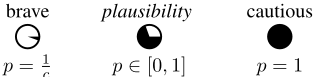
However, these simple reasoning modes are insufficient if we are interested in more fine-grained reasoning, for example, the probability of an atom occurring in an answer set. More generally, we say plausibility reasoning asks whether a set Q of literals matches at least p · 100% of the answer sets for p ∈ [0, 1]. Figure 1 illustrates this more fine-grained reasoning mode between brave and cautious reasoning for the program Π in focus and the query Q and probability p of interest. To obtain the present probability to answer the matching question, we need to count the total number c of answer sets and the number of answer sets under the query.
In the ASP community, compact problem modeling is seen as an advantage of the formalism. Modeling oftentimes requires to introduce auxiliary atoms into the program. If these atoms are functionally independent of the atoms of interest, we need to hide the auxiliary atoms. In our setting, this yields plausibility under projection of atoms of interest and plausibility reasoning under projection. To obtain the projected plausibility, we relate the total number of answer sets projected to the atoms of interest, called projected counting or #PAs for short, and the number of answer sets projected to the atoms of interest under the query. When handling decision problems we can simply ignore auxiliary atoms. In contrast, when dealing with plausibility, need to treat multiple answer sets that are identical on the atoms of interest as one answer set making the problem harder to solve. This is also justified by complexity theoretical considerations, namely, counting answer sets is #·co-NP-complete, projected answer set counting is #·ΣP 2 -complete dropping to #·co-NP if all atoms are taken as projected atoms [Fichte and Hecher, 2019].
In practice, counting becomes quickly impractical with standard systems such as clasp. Instead, we present a novel hybrid approach for plausibility reasoning under projections, which relies on projected answer set counting as basis.
Contributions. Our main contributions are as follows.
- We formally introduce the fine-grained reasoning mode plausibility reasoning under projection to ASP.
- We combine existing systems with fast dynamic programming into a hybrid solver for plausibility reasoning.
- We provide an implementation and initial empirical evaluation. In our experiments, we see feasibility and advantages of our approach over existing ASP systems.
Related Work. Gebser, Kaufmann and Schaub [Gebser et al., 2009] considered projected enumeration for ASP. For plain answer set counting, several techniques have been developed, e.g. [Aziz et al., 2015; Jakl et al., 2009], including epistemic extensions and quantitative reasoning [Besin et al., 2021]. Systems and techniques for probabilistic reasoning have been studied (see, e.g. [Baral et al., 2009; Fierens et al., 2015; Lee et al., 2017; Riguzzi and Swift, 2018; Eiter et al., 2021]). P-log combines ASP with causal Bayesian networks [Baral et al., 2009]. ProbLog uses probabilistic facts and the well-founded semantics [Fierens et al., 2015]. LP MLN [Lee et al., 2017] has decision-based notions of relative occurrences of answer sets and their weights. For projected counting, parameterized algorithms for treewidth have been studied in theory [Fichte and Hecher, 2019]. For a survey on propositional counting see [Fichte et al., 2021a].
2 Preliminaries
Answer Set Programming (ASP). We follow standard definitions of propositional ASP [Marek and Truszczynski, 1999; Niemel¨a, 1999]. Let ℓ, m, n be non-negative integers such that ℓ ≤ m ≤ n, a1, . . ., an be distinct atoms. We refer by literal to an atom or the negation thereof. A program Π is a finite set of rules of the form a1 ∨ · · · ∨ aℓ ← aℓ+1, . . . , am, ¬am+1, . . . , ¬an. For a rule r, we let Hr := {a1, . . . , aℓ}, B+ r := {aℓ+1, . . . , am}, and Br := {am+1, . . . , an}. We denote the sets of atoms occurring in a rule r or in a program Π by at(r) := Hr ∪ B+ r ∪ Br and at(Π) := ∪r∈Π at(r). Let Π be a program and Q be a set of literals (query). Then, Π⊔Q := Π∪ {← ¬a,← b | a ∈ Q∩ at(Π), ¬b ∈ Q} is the program Π under Q. An interpretation I is a set of atoms. We define I := {¬a | a ∈ I} and say that Q matches I, if Q ∩ at(Π) = I and Q ∩ I = ∅. I satisfies a rule r if (Hr ∪ Br ) ∩ I ̸= ∅ or B+ r \I ̸= ∅. I is a model of Π if it satisfies all rules of Π. The Gelfond-Lifschitz (GL) reduct of Π under I is the programΠI obtained fromΠ by first removing all rules r with Br ∩I ̸= ∅ and then removing all ¬z where z ∈ Br from the remaining rules r [Gelfond and Lifschitz, 1991]. I is an answer set of a program Π, in symbols I |= Π, if I is a minimal model of ΠI . The set of answer sets are given by AS(Π) := {I ⊆ at(Π) | I |= Π}. Deciding whether a disjunctive program has an answer set is ΣP 2 -complete [Eiter and Gottlob, 1995]. The problem is called consistency of an ASP program. For restricted forms, the complexity drops to NP-complete [Marek and Truszczy´nski, 1991]. If AS(Π) = ∅, we say Π is inconsistent.
Example 2. Consider Π from Example 1 and its three answer sets as well as the projection P := {a, b}. When we project the answer sets to P, we only have the two answer sets {a} and {b}, i.e., the projected answer set count #PA(Π, P) is 2.
Example 1. Consider the program Π := {a ∨ b ←; c ← ¬d; c ∨ d ← b; }. Answer sets of Π are {a, c}, {b, c}, and {b, d}. Projected Answer Set Counting (#PA). Let Π be a program and P be a set of atoms, called projection. Then, projected answer set counting #PA on Π and P is the number of subsets I ⊆ P s.t. I ∪ J is an answer set of Π for some set J ⊆ at(Π) \ P, i.e., #PA(Π, P) := |{I ∩ P | I |= Π}|. Problem #PA(Π, A) is #·ΣP 2 -complete.
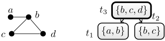
Tree Decompositions (TDs). We follow standard terminology on graphs and digraphs. For a tree T with root root(T) and a node t of T , we let children(t, T ) be the set of all child nodes t′ of t. Let G = (V,E) be a graph. A tree decomposition (TD) of graph G is a pair T = (T, χ), where T is a rooted tree, and χ a mapping that assigns to each node t of T a set χ(t) ⊆ V , called a bag, such that the following conditions hold: (i) V = ⋃t of T χ(t) and E ⊆ ⋃t of T {{u, v} | u, v ∈ χ(t)}; and (ii) for each r, s, t, such that s lies on the path from r to t, we have χ(r) ∩ χ(t) ⊆ χ(s). Then, width(T ) := maxt of T |χ(t)| - 1. The treewidth tw(G) of G is the minimum width(T ) over all TDs T of G. For arbitrary but fixed w ≥ 1, it is feasible in linear time to decide if a graph has treewidth at most w and, if so, to compute a TD of width w [Bodlaender and Kloks, 1996].
For the ease of presentation, we use nice TDs, which can be computed in linear time without increasing the width [Bodlaender and Kloks, 1996] and are defined as follows. For a node t ∈ N, we say that type(t) is leaf if children(t, T) = ⟨⟩; join if children(t, T) = ⟨t′ , t′′ ⟩ where χ(t) = χ(t′ ) = χ(t′′ ) ̸= ∅; intr ("introduce") if children(t, T) = ⟨t′ ⟩, χ(t′ ) ⊆ χ(t) and |χ(t)| = |χ(t′ )| + 1; rem ("removal") if children(t, T ) = ⟨t′ ⟩, χ(t′ ) ⊇ χ(t) and |χ(t′ )| = |χ(t)| + 1. If for every node t ∈ N, type(t) ∈ {leaf, join, intr, rem}, and χ(t′ ) = ∅ for root and leaf t′ , the TD is nice.
In order to use TDs for ASP, we define the primal graph GΠ of a program Π [Jakl et al., 2009], which has vertices the atoms of Π with an edge {a, b} whenever there exists a rule r ∈ Π s.t. a, b ∈ at(r).
Example 3. Figure 2 illustrates the primal graph GΠ of Π from Example 2 as well as a tree decomposition of GΠ of width 2, which is also the treewidth of GΠ.
Dynamic Programming (DP). Tree Decompositions enable dynamic programming algorithms, whose effort is (exponentially) bounded by the width of a TD. These algorithms take a TD T = (T, χ) of a given instance (graph), and iterate over every node of T in post-order, i.e., they perform a bottom-up traversal of T. Thereby, for each node t of T during the traversal, an algorithm is executed that computes a table τt for t, which is a set of sequences that are partial solutions to a local problem restricted to the bag χ(t). For ASP, we define these local problem by DP program Πt := {r ∈ Π | at(r) ⊆ χ(t)}. Such DP algorithms are exponential only in the largest bag size, which allow for efficient counting without explicitly enumerating all solutions.
3 Plausibility Reasoning via Projection
Recall that the ASP literature distinguishes the traditional reasoning modes, cautious (skeptical) and brave (credulous) reasoning. Both modes consider a given program Π as well as a set Q of literals. Cautious reasoning then asks whether query Q matches every answer set of Π, whereas brave reasoning focuses only on determining whether Q matches some answer set of Π. Interestingly, both ASP reasoning modes are extreme forms of its own, since cautious reasoning is rather strict or unlikely to hold in general, whereas brave reasoning is very easy to be answered affirmatively, cf. Figure 1.

Example 4. Recall Π from Example 1 and observe that brave reasoning on {a}, {b}, {c}, or {d} is answered affirmatively, which is not the case for cautious reasoning.
Towards providing more fine-grained reasoning modes, we measure the proportion of answer sets matching query Q. Formally, we define the plausibility of Q as the proportion of answer sets matching Q.
Definition 1 (Projected Plausibility). Let Π be a program, Q be a query, and P be projection. Then, (P-)projected plausibility of ΠunderQ is defined P[Π,Q]|P := #PA(Π⊔Q,P) max(1,#PA(Π,P )) .
Note that the usage of max prevents division by zero, i.e., in case of consistency plausibility is zero as well. Interestingly, with the help of plausibility, one can define a more fine-grained reasoning mode that generalizes and subsumes both cautious and brave reasoning.
Definition 2 (Plausibility Reasoning). Let Π be a program, Q be a set of literals, P be a set of atoms, and 0≤p≤1. Then, plausibility reasoning on Q and p asks if P[Π, Q]|P ≥ p.
Example 5. Plausibility reasoning on a program Π provides more fine-grained reasoning between the two extreme cases of cautious reasoning (p= 1 | at(Π)| ) and brave reasoning (p = 1), where P = at(Π). In our running example, P[Π, {b}]at(Π) = P[Π, {c}]at(Π) = 2 3 , which could show that b and c are very likely (compard to, e.g. P[Π, {a}]at(Π) = 13 ). This might suffice in drawing conclusions based on quantitative arguments. However, assuming that a and b are atoms of interest, indicating that plausibility should be considered using projection P = {a, b} of Example 2, it turns out that P[Π, {a}]P = P[Π, {b}]P = 1 2 . Interestingly, P[Π, {c}]P = 1, since the answer sets matching {c} when projected to P are identical to AS(Π) restricted to P. As a consequence, P[Π, {c}]P is more likely than P[Π, {b}]P , since Π under query {c} leads to every projected answer set of Π and P .
In order to efficiently perform plausibility reasoning, we need a fast implementation of projected answer set counting, which we pursue in the following.
3.1 Towards a Hybrid Approach for Plausibility
While existing answer set solvers showed a tremendous performance increase in the last decades, counting requires different techniques, especially if the number of solutions is beyond the limit of enumeration. Over the time, some approaches have been lifted from Boolean satisfiability to ASP (e.g. [Jakl et al., 2009; Pichler et al., 2010; Eiter et al., 2021; Besin et al., 2021]). However, those are not available for counting with respect to projection (#PA), which, as indicated in the preliminaries, is probably harder than plain counting. We propose a new method, that is hybrid in the sense that it combines ideas from parameterized complexity with standard ASP solving, thereby providing a flexible balance between those. Inspired by existing works [Eiben et al., 2021; Dell et al., 2019; Hecher et al., 2020], we define a graph representation that will be used to combine these ideas.

Definition 3. Let Π be a program and A ⊆ at(Π). A projection path (in GA Π ) is a path in GΠ of the form a, c1, . . . , cℓ, b s.t. {a, b} ⊆ A, ℓ ≥ 0, and {c1, . . . , cℓ}∩A = ∅. The projection primal graph GA Π has A as vertices with an edge between two a, b ∈ A, whenever there is a projection path from a to b.
Example 6. Recall Π and projection P from Example 2. Figure 3 shows projection primal graphs G PΠ (left), G {b,c} Π (middle), and G {a,c,d} Π (right) with an edge {a, c} due to projection path a, b, c and an edge {a, d} due to projection path a, b, d.
Interestingly, this projection graph provides the flexibility to decide the balance between dynamic programming and standard solving. If we choose for A = ∅, we obtain by GAΠ the empty graph, i.e., all the effort goes to standard solving with no focus on dynamic programming, whereas A = at(Π) yields the primal graph GAΠ = GΠ for full dynamic programming. We make this precise, by formalizing "effort" in terms of ASP programs that are needed to be solved.
Definition 4. Let Π be a program and A ⊆ at(Π). Further, assume a TD T =(T, χ) of GA Π , and a node t of T. Then, the sub atoms (at t) are given by χAt :={x∈ at(Π) \ A | x /∈ ⋃t′ of T,t′ ̸=t χAt′ , {a, b} ⊆ χ(t), x is in a projection path of GA Π from a to b}. The sub program(at t) is definedΠAt :={r∈Π\Πt | at(r)⊆χAt ∪χ(t)}.
Note that there are many possibilities to fulfill sub atoms of Definition 4, which can be treated differently in actual implementations. Observe that for the primal graph G ∅Π = GΠ, the sub program at any node is empty, wheras for the empty graph G at(Π) Π and a TD thereof consisting only of one node t has ΠAt = Π. Intuitively, the set A and these definitions provide us a "handle" to share and shift complexity between dynamic programming (DP program Πt) and standard solving (sub program ΠAt ). As a result, we refer to crucial set A by (projection) abstraction.
Example 7. Recall projection primal graphs G {b,c} Π and G {a,c,d} Π of Figure 3. Compare primal graph vs. projection graph. Figure 4 shows a TD T1 of G {b,c} Π and a TD T2 of G {a,c,d} Π . The sub programs for T1 could be defined by Π{b,c} t1 :={a∨b ←} and then Π{b,c} t2 :={c ←¬d, c ∨d ← b}. Alternatively, one can also fulfill Definition 4 by setting Π{b,c} t1 to the empty set and Π{b,c} t2 to Π. In any case, for T1 the main effort goes into the sub programs, since the DP programs are empty. This is in contrast to T2, where we
In: Depth dpth ≥ 0, program Π, projection P , and a query Q. Out: The plausibility P(Π, Q)|P . 1 A←P 2 cn ←AS(Π)̸=∅ /* Standard ASP */ 3 if A=∅ or cn=0/*∅ Projection / Inconsistent*/ then return cn · (AS(Π ⊔ Q) ̸= ∅) 4 T = (T, χ) ←Decompose(GA Π) /* Heuristics */ 5 if width(T ) ≥ thresholdhybrid or dpth ≥ 2 then 6 return #PA(Π⊔Q,P) max(1,#PA(Π,P)) /* Standard Solver */ 7 if width(T ) ≥ thresholdabstr /* Abstraction */ then 8 A ← Choose-Abstraction(A, Π) 9 T = (T, χ) ←Decompose(GA Π ) 10 for t in post-order(T)/*Dynamic Programming*/do 11 Child-Tabs ← ⟨τt1 , . . . , τtℓ ⟩ where children(t)=⟨t1, . . . , tℓ⟩ 12 τt ←PAt(dpth, χ(t),Πt,ΠAt , P,Q, Child-Tabs) 13 return ∑⟨I,q,c⟩∈τroot(T),c>0 qc /* Plausibility */see a different balance between DP and sub programs, having DP program Πt1 ={c ← ¬d} and sub program Π{a,c,d} t1 = {a ∨ b ←, c ∨ d ← b}, which is the only possibility for T2 to ensure Definition 4. Observe that while the assignment of sub programs for nodes is flexible, set A in Definition 4 uniquely partitions between all DP programs and all sub programs.
For the sake of simpler algorithms, in constrast to, e.g., [Fichte and Hecher, 2019], from now on we assume safe programs Π and projections P that ensure: (i) every DP program Πt contains every rule, whose head intersects with P ∩ χ(t), i.e., Πt ⊆ {r ∈ Π | Hr ∩P ∩χ(t) ̸= ∅} and (ii) no cyclic dependency (cycle in positive dependency graph) among atoms in P. This is not a strong restriction that is fulfilled, e.g., via free "choices" on auxiliary atoms by usingP ′ :={a′ | a ∈ P} and Π′ :=Π∪{{a′ } ←;← a′ , ¬a;← ¬a′ , a | a ∈ P} instead.
3.2 Plausibility by means of Hybrid Solving
The algorithm for hybrid solving is outlined in Listing 1, taking a given depth dpth (initially 0), a program Π, and a projection P, which we assume in this section. Listing 1 consists of four blocks. The first block spans Lines 1-3, which initially takes as abstraction A the projection P and checks whether Π is consistent. If either the projection is empty or Π is inconsistent, we can return the result immediately. In the second block consisting of Lines 4-6, we decompose GΠ via heuristics, thereby obtaining TD T . If the width of computed T is larger than thresholdhybrid or the depth dpth is out of reach, we solve the problem via an existing standard solver. Otherwise, we use dynamic programming, where the third block consisting of Lines 7-9 seeks for a suitable abstraction A ⊆ P, if this seems promising, i.e., if width(T ) is larger than thresholdabstr. Note that if the width is below thresholdabstr, we have that A = P and therefore G A Π = G PΠ . The abstraction in Line 8 can be obtained heuristically, which in our implementation is achieved by means of an ASP encoding using optimization. Details on our implementation will be discussed in Section 4. After obtaining such an abstraction A, Line 9 computes a TD of G A Π and assigns it to T .
Listing 2: Table algorithm PAt(dpth, χt,Πt,ΠAt , P,Q ⟨τ1, . . . , τℓ⟩) for nice TDs of the projection primal graph. In: Depth dpth ≥ 0, bag χt, program Πt, sub program ΠAt , projection P , query Q, and child tables ⟨τ1, . . . , τℓ⟩ of t. Out: Table τt. 1 if type(t) = leaf then τt ← {⟨∅, 1, 1⟩} 2 else if type(t) = intr and a∈χt is introduced then 3 τt ← {⟨J, q′ , c′ ⟩ | ⟨I, q, c⟩ ∈ τ1, J∈{I, I ∪{a}}, J |= Πt, 4 q′=q · HybPA(dpth+1,Π′⊔Q, P,Q),Π′=(ΠAt ∪J), 5 c′=c · HybPA(dpth+1,Π′ , P,Q), q′ > 0, c′ > 0} 6 else if type(t) = rem and a ̸∈ χt is removed then 7 τt ← {⟨I ′ , ∑⟨J,q′,c′⟩∈τ1:I′\{a}=J q′ , ∑⟨J,q′,c′⟩∈τ1:I′\{a}=J c′ ⟩ | ⟨I, q, c⟩ ∈ τ1, I ′ = I \ {a}} 8 else if type(t) = join then 9 τt ← {⟨I, q1 · q2, c1 · c2⟩ | ⟨I, q1, c1⟩ ∈ τ1, ⟨I, q2, c2⟩ ∈ τ2} 10 return τtFinally, the last block performs the actual dynamic programming on the projection graph GA Π , which spans Lines 1012. Thereby, Line 10 takes the current TD T = (T, χ) and iterates though every node of T in post-order. For each node t of T during the traversal, an algorithm PAt is executed, computing a table τt for t, which is a set of sequences of the form ⟨I, q, c⟩, where I ⊆ χ(t) is an interpretation restricted to χ(t) and q, c are integers used for counting (counters). Precisely, q is the projected answer set count of the program Π′ under Q, where Π′ contains all DP programs and sub programs for every node below t under I. So, q = #PA(Π′ ⊔ (Q∪I), P) and c is the projected answer set count of Π′ , i.e., c = #PA(Π′ , P). Observe that therefore these counters for the root table lead to the projected plausibility of the whole program. In Line 12, PAt gets as parameters dpth, the bag, DP program Πt, sub program ΠAt , projection P , query Q, and tables for all child nodes of t.
The algorithm PAt is given in Listing 2, which we briefly discuss. For the ease of presentation, PAt assumes that the used TD T is nice, i.e., it gives a clear case distinction between nodes of types leaf, intr, rem, and join. Note that the usage of nice TDs is not a restriction, since one can overlap these cases accordingly in order to obtain an algorithm for a node of an arbitrary TD. For (empty) leaf nodes, in Line 1 we construct the empty interpretation and set both counters to 1. Then, when an atom a ∈ χt is introduced in Line 2, in the current branch of the tree, a is encountered for the first time. Consequently, interpretation J extends I by either including a or not, and we ensure in Line 3 that J is an answer set of DP program Πt. Line 4 (recursively) calls agorithm HybPA on the increased depth, for obtaining the projected count on the sub program Π′ under Q. Line 5 computes the regular projected count on Π′ , through recursion via agorithm HybPA. Since, intuitively, the computed counts form "sub problems", we merge the resulting counts by multiplication and only keep positive numbers. Further, whenever an atom a gets removed in Line 6, it is guaranteed by the properties of a TD that every rule containing a has been processed. As a result, we remove a from the interpretation and potentially merge counts of interpretations that then coincide by taking the sum (cf. Line 7). Finally, when joining nodes of different (independent) branches, the counters of matching interpretations are multiplied, as shown in Line 9.
Theorem 1 (Correctness). Algorithm HybPA is correct. Precisely, for every given safe program Π and projection P , and query Q, we have that HybPA(0, Π, P, Q) returns P(Π, Q)|P . Proof (Sketch). We present the proof outline for a slightly stronger statement, where for any query R we show correctness: HybPA(dpth, Π⊔R, P, Q) = P(Π⊔R, Q)|P . For showing correctness of HybPA(dpth, Π⊔R, P, Q) for any dpth ≥ 0, we perform structural induction, where we assume induction hypothesis H: Correctness of HybPA(dpth+1, Π′ ∪ R′ , P, Q) for any Π′ ⊆ Π and any query R′ .
For showing soundness of PAt, we define the following invariant I for any node t of T : The sequence ⟨I, q, c⟩ returned by PAt ensures that q amounts to #PA(Π′ ⊔ Q, P) and c amounts to #PA(Π′ , P), where Π′ is the whole program of the subtree below t, i.e., Π′ := ⋃t′ of T,t′ below t (Πt ∪ ΠAt ). Observe that therefore if I holds, Line 13 returns P(Π, Q)|P .
We show that HybPA(dpth,Π, P,Q) always returns P(Π,Q)|P . Observe that in case of empty projections P, cn · (AS(Π⊔Q)̸=∅) = AS(Π⊔Q)̸=∅ max(1,AS(Π)̸=∅) since cn = 0 (inconsistency of Π) implies that also Π⊔Q is inconsistent (Q only adds constraints, i.e., rules with empty heads). Consequently, Line 3 of Listing 1 returns the projected plausibility. Line 6 fulfills Definition 1 as well. For the soundness of dynamic programming, assume a set A ⊆ P and a TD T = (T, χ) of G A Π . By Definition 4, each atom x ∈ at(Π) \ A appears among sub atoms χAt for at most one node t of T. Further, by construction of G A Π (cf. Definition 3) there always exists a projection path containing x. Consequently, there is a unique node t s.t. x ∈ χAt and we follow that for every rule r ∈ Π there is a unique node t of T with either r ∈ Πt or r ∈ ΠAt .
The invariant I can be shown by structural induction on T , whereby we prove it for any node t of T of type type(t) ∈ {leaf, intr, rem, join}, thereby assuming I for every child node of t. The remainder is a technical case distinction for type(t) ∈ {leaf, intr, rem, join}. Note that for type(t) = intr and Lines 4 and 5, we apply induction hypothesis H, thereby concluding correctness of the calls to HybPA.
4 Implementation and Experimental Results
We implemented algorithm HybPA, as given in Listings 1 and 2, into the system HybPA, which is publicly available at https://github.com/maliabd-al-majid/dpdb ASP. Our system builds upon clingo 5.5.1 [Gebser et al., 2009] and the tool dpdb [Fichte et al., 2021b] for handling table manipulations during dynamic programming via database management system PostgreSQL version 12.9. HybPA is written in Python3 and uses the decomposition tool htd [Abseher et al., 2017] to efficiently obtain TDs (not necessarily nice) via heuristics.
Implementation Details. We briefly discuss implementation specifics along the lines of Listing 1. In Line 2, we call clingo. Since we anyways need the solving call to decide consistency, we extend this in practice and let clingo run for 60 seconds. If the plausibility is already solved by clingo, we stop and output the result. Lines 4 and 9 use htd to decompose heuristically. The constant thresholdhybrid is set to 1000 and thresholdabstract is set to 8, allowing for aggressive abstractions. Then, for solving projected counting, Line 6 invokes clingo with options "-q" and "--project", where projection P is set via statements "#show" in the encoding. The computation of suitable abstractions A ⊆ P in Line 8 is implemented using two ASP encodings that are solved by means of clingo. In details, we developed a twophase approach via heuristics, due to some large instances: First, we estimate among P up to 95 elements of smallest degree, for which we use up to 10 seconds and interrupt afterwards, taking the best result found. Then, among those 95 elements, we invest up to 35 seconds for finding up to 64 elements for the final abstraction. Thereby, we approximate those elements, which lead to a projection primal graph of small width. Both encodings were implemented using weak constraints (optimization), interrupting the computation after the respective timeouts. For details, we refer to the encodings of the supplemental material. The table algorithm of Line 12, i.e., Algorithm PAt of Listing 2, is implemented using PostgreSQL, which is based on relational algebra. Thereby, the construction of the sub program for a node (cf. Definition 4) in Line 12 is implemented such that TD nodes lower in the tree get precedence, i.e., we prefer larger sub programs lower than higher in the tree.
Experimental Setting and Instances. Our main interest are more fine-grained reasoning modes between simple brave and cautious reasoning. In order to evaluate practical feasibility, we conducted a series of practical experiments. Computing projected plausibility for a query mainly relies on projected answer set counting for a program and a given projection. Since #PA(Π, P) is the computationally hardest part being #·ΣP 2 -complete, we focus on this part in our experimental evaluation without explicitly assuming queries. In the following, we state two hypotheses that we aim to study and verify in the course of our experimental analysis.
- H1: We can compute projected answer sets for a large part of crucial problems in ASP allowing for projected plausibility reasoning in ASP.
- H2: Hybrid solving using HybPA outperforms clingo, in particular, on hard instances.
No dedicated projected answer set counter exist. But the system clingo can solve #PA [Gebser et al., 2009], which we take for comparison. As instances, we take two sets (S1) ASP instances from the abstract argumentation competition and (S2) a prototypical ASP domain with reachability and use of transitive closure on real-world graphs. In more details, S1 contains instances of the ICCMA'17 competition [Lagniez et al., 2021]. We focused on the 2017 instances, since the ICCMA'19 instances are known to be on the easier side and the ICCMA'21 can be tackled well by non-hybrid dynamic programming [Lagniez et al., 2021]. The ASP encoding for admissible extensions was taken from the ASPARTIX system [Dvoˇr´ak et al., 2020]. On the ICCMA'17 instances, we create 4 subsets by randomly selecting 25, 50, 75, and 100 projection atoms. For S2, we used real-world graphs of public transport networks from all over the world, which were used in the PACE'16 and '17 challenges [Dell et al., 2017]. In total, the transit instances consist of 561 full networks and 2553 subgraphs with different transportation modes. For each instance, we assume the station with the smallest and largest index to be the start and end stations, respectively. We randomly selected 25 atoms for projection.
| Set | System | n | t[h] | tAvg [s] |
|---|---|---|---|---|
| S1 | clingo | 1797 | 683.6 | 49.17 |
| HybPA | 1913 | 628.1 | 90.46 | |
| vbest | 1929 | 622.0 | 53.53 | |
| S2 | clingo | 1087 | 117.2 | 28.66 |
| HybPA | 1146 | 89.5 | 32.88 | |
| vbest | 1150 | 87.5 | 32.79 |
Platform, Measure, and Restrictions. All our solvers ran on a cluster consisting of 12 nodes. Each node of the cluster is equipped with two Intel Xeon E5-2650 CPUs, where each of these 12 physical cores runs at 2.2 GHz clock speed and has access to 256 GB shared RAM. Results are gathered on Ubuntu 16.04.1 LTS powered on kernel 4.4.0-139 with hyperthreading disabled using version 3.7.6 of Python3. We mainly compare wall clock time. Run times larger than 1,800 seconds, respectively, count as timeout and main memory (RAM) was restricted to 60GB. We ran jobs exclusively on one machine, where solvers were executed sequentially with exclusive access and no parallel execution of other runs.
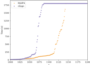
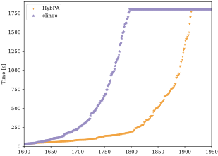
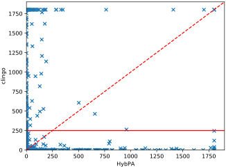
Experimental Results and Summary. Figure 5 (left) and (middle) illustrates the number of solved instances for the sets S1 (argumentation) and S2 (reachability) as cactus plot. In addition, Figure 5 (right) visualizes the solved instances for clingo vs HybPA in a direct comparison on set S2. Notably, HybPA solved instances for which the decomposer constructed a decomposition of up to width 100. The detailed results in Table 1 show that a notable number of instances can be solved, which confirms H1. In fact, HybPA completes clasp by allowing to solve a notable number of instances more, both on S1 and S2. Unsurprisingly, the total runtime is quite high for this computationally very hard problem. clingo solves instances with few solutions fast. Average runtime indicates that HybPA tackles harder instances. In particular, we see that HybPA works well on instances with a large number of projected answer sets. Indeed, nested solving outperforms clingo (H2) on both instance sets. The performance gain of HybPA is especially visible in Figure 5. There the rightmost subfigure illustrates a scatter plot. In fact, all instances solved below the dashed line can already be solved by clingo, which hybrid solving can easily take advantage of by appropriate parameter tuning. Instead, we see that a notable number of instances is above the identity line meaning that HybPA can solve those instances while clingo solves only few instances that cannot be solved by hybrid solving.
5 Conclusion and FutureWork
This work introduced a more fine-grained reasoning mode for answer set programming (ASP) that is between cautious and brave reasoning. In addition to these, plausibility reasoning allows to draw conclusion based on the the actual (quantitative) proportion, a given query Q holds. This is visualized in Figure 1 and can be seen as an alternative for drawing conclusions in logic programs, if both cautious and brave reasoning are too weak and too strict, respectively.
In order to provide the flexibility to pull focus or concentrate on variables V of interest (unaffected by encodings involving auxiliary variables), we base plausibility reasoning on the framework of projected model counting, reasoning over answer sets with respect to V . Due to the lack of existing (projected) counting systems for ASP, we developed a novel hybrid approach that interleaves ideas from parameterized algorithmics (dynamic programming on tree decompositions) and standard CDCL-based solving. This concept uses dedicated abstractions in order to speed-up CDCL-based search via DP algorithms suitable for counting. Our experimental results confirm that this is indeed promising.
For future work, we plan to tightly integrate our method into ASP solvers. We expect that multi-shot extensions of ASP enable advanced learning, by unifying solver entities and sharing learned constraints (nogoods) among different tree decompositions nodes. Further, we are convinced that approximate variants of plausibility reasoning that do not precisely compute plausibility [Kabir et al., 2022], could provide a fruitful alternative for computationally hard applications.
Acknowledgments
This research has been supported by the Vienna Science and Technology Fund (WWTF) grant ICT19-065, and by the Austrian Science Fund (FWF) grants P32830 and Y698.
@inproceedings{ijcai2022p363,
  title     = {Plausibility Reasoning via Projected Answer Set Counting - A Hybrid Approach},
  author    = {Fichte, Johannes K. and Hecher, Markus and Nadeem, Mohamed A.},
  booktitle = {Proceedings of the Thirty-First International Joint Conference on
               Artificial Intelligence, {IJCAI-22}},
  publisher = {International Joint Conferences on Artificial Intelligence Organization},
  editor    = {Luc De Raedt},
  pages     = {2620--2626},
  year      = {2022},
  month     = {7},
  note      = {Main Track},
  doi       = {10.24963/ijcai.2022/363},
  url       = {https://doi.org/10.24963/ijcai.2022/363},
}
TY - CPAPER TI - Plausibility Reasoning via Projected Answer Set Counting - A Hybrid Approach AU - Fichte, Johannes K. AU - Hecher, Markus AU - Nadeem, Mohamed A. T2 - Proceedings of the Thirty-First International Joint Conference on Artificial Intelligence, IJCAI-22 PB - International Joint Conferences on Artificial Intelligence Organization PY - 2022 SP - 2620 EP - 2626 DO - 10.24963/ijcai.2022/363 UR - https://doi.org/10.24963/ijcai.2022/363 ER -Copied
Machine-readable versions of this paper, for tools and AI agents:





