
Neural Contextual Anomaly Detection for Time Series
Proceedings of the Thirty-First International Joint Conference on Artificial Intelligence. Main Track. Pages 2843-2851.
https://doi.org/10.24963/ijcai.2022/394
Keywords
- Data Mining: Anomaly/Outlier Detection
- Machine Learning: Time-series; Data Streams
Abstract
We introduce Neural Contextual Anomaly Detection (NCAD), a framework for anomaly detection on time series that scales seamlessly from the unsupervised to supervised setting, and is applicable to both univariate and multivariate time series. This is achieved by combining recent developments in representation learning for multivariate time series, with techniques for deep anomaly detection originally developed for computer vision that we tailor to the time series setting. Our window-based approach facilitates learning the boundary between normal and anomalous classes by injecting generic synthetic anomalies into the available data. NCAD can effectively take advantage of domain knowledge and of any available training labels. We demonstrate empirically on standard benchmark datasets that our approach obtains a state-of-the-art performance in the supervised, semi-supervised, and unsupervised settings.
- [Aubet et al., 2021] Franc ¸ois-Xavier Aubet, Daniel Zügner, and Jan Gasthaus. Monte carlo em for deep time se- ries anomaly detection. arXiv preprint arXiv:2112.14436, 2021.
- [Audibert et al., 2020] Julien Audibert, Pietro Michiardi, Frédéric Guyard, Sébastien Marti, and Maria A Zuluaga. Usad: Unsupervised anomaly detection on multivariate time series. In 26th ACM SIGKDD, 2020.
- [Ayed et al., 2020] Fadhel Ayed, Lorenzo Stella, Tim Januschowski, and Jan Gasthaus. Anomaly detection at scale: The case for deep distributional time series models. arXiv preprint arXiv:2007.15541, 2020.
- [Bock et al., 2022] Christian Bock, Franc ¸ois-Xavier Aubet, Jan Gasthaus, Andrey Kan, Ming Chen, and Laurent Cal- lot. Online time series anomaly detection with state space gaussian processes. arXiv preprint arXiv:2201.06763, 2022.
- [Breunig et al., 2000] Markus M Breunig, Hans-Peter Kriegel, Raymond T Ng, and Jörg Sander. Lof: iden- tifying density-based local outliers. In ACM SIGMOD, 2000.
- [Ehrlich et al., 2021] Elena Ehrlich, Laurent Callot, and Franc ¸ois-Xavier Aubet. Spliced binned-pareto distribu- tion for robust modeling of heavy-tailed time series. arXiv preprint arXiv:2106.10952, 2021.
- [Franceschi et al., 2019] Jean Yves Franceschi, Aymeric Dieuleveut, and Martin Jaggi. Unsupervised scalable rep- resentation learning for multivariate time series. In Pro- ceedings of the 33th Conference on Neural Information Processing Systems, NeurIPS, 2019.
- [Gao et al., 2020] Jingkun Gao, Xiaomin Song, Qingsong Wen, Pichao Wang, and et al. RobustTAD: Ro- bust Time Series Anomaly Detection via Decomposi- tion and Convolutional Neural Networks. arXiv preprint arXiv:2002.09545, 2020.
- [Hendrycks et al., 2019] Dan Hendrycks, Mantas Mazeika, and Thomas Dietterich. Deep anomaly detection with out- lier exposure. In ICLR, 2019.
- [Hundman et al., 2018] Kyle Hundman, Valentino Con- stantinou, Christopher Laporte, Ian Colwell, and Tom Soderstrom. Detecting spacecraft anomalies using lstms and nonparametric dynamic thresholding. In 24th ACM SIGKDD, 2018.
- [Kim et al., 2022] Siwon Kim, Kukjin Choi, Hyun-Soo Choi, Byunghan Lee, and Sungroh Yoon. Towards a rig- orous evaluation of time-series anomaly detection. In Pro- ceedings of the 36th AAAI Conference on Artificial Intelli- gence, AAAI-22, 2022.
- [Lavin and Ahmad, 2015] Alexander Lavin and Subutai Ah- mad. Evaluating real-time anomaly detection algorithms- the numenta anomaly benchmark. In IEEE 14th ICMLA, 2015.
- [Li et al., 2019] Dan Li, Dacheng Chen, Baihong Jin, Lei Shi, Jonathan Goh, and See-Kiong Ng. Mad-gan: Mul- tivariate anomaly detection for time series data with gen- erative adversarial networks. In ICANN, 2019.
- [Liu et al., 2008] Fei Tony Liu, Kai Ming Ting, and Zhi-Hua Zhou. Isolation forest. In 2008 eighth ieee international conference on data mining. IEEE, 2008.
- [Liu et al., 2015] Dapeng Liu, Youjian Zhao, Haowen Xu, Yongqian Sun, and et al. Opprentice: Towards practical and automatic anomaly detection through machine learn- ing. In Proceedings of the 2015 Internet Measurement Conference, 2015.
- [Park et al., 2018] Daehyung Park, Yuuna Hoshi, and Charles C Kemp. A multimodal anomaly detector for robot-assisted feeding using an lstm-based variational au- toencoder. IEEE Robotics and Automation Letters, 2018.
- [Ren et al., 2019] Hansheng Ren, Bixiong Xu, Yujing Wang, Chao Yi, and et al. Time-Series Anomaly Detection Ser- vice at Microsoft. In 25th ACM SIGKDD, 2019.
- [Ruff et al., 2018] Lukas Ruff, Robert A Vandermeulen, Nico Görnitz, Lucas Deecke, and et al. Deep One-Class Classification. In ICML, 2018.
- [Ruff et al., 2020a] Lukas Ruff, Robert A Vandermeulen, Billy Joe Franks, Klaus-Robert Müller, and Marius Kloft. Rethinking assumptions in deep anomaly detection. arXiv preprint arXiv:2006.00339, 2020.
- [Ruff et al., 2020b] Lukas Ruff, Robert A Vandermeulen, Nico Görnitz, Alexander Binder, and et al. Deep Semi- Supervised Anomaly Detection. In ICLR, 2020.
- [Ruff et al., 2021] Lukas Ruff, Jacob R. Kauffmann, Robert A. Vandermeulen, Gregoire Montavon, and et al. A Unifying Review of Deep and Shallow Anomaly Detection. Proceedings of the IEEE, 2021.
- [Schlegl et al., 2017] Thomas Schlegl, Philipp Seeböck, Se- bastian M Waldstein, Ursula Schmidt-Erfurth, and Georg Langs. Unsupervised anomaly detection with generative adversarial networks to guide marker discovery. In Inter- national conference on information processing in medical imaging, 2017.
- [Schölkopf et al., 1999] Bernhard Schölkopf, Robert C Williamson, Alexander J Smola, John Shawe-Taylor, John C Platt, et al. Support vector method for novelty detection. In NIPS 12, 1999.
- [Shen et al., 2020] Lifeng Shen, Zhuocong Li, and James Kwok. Timeseries anomaly detection using temporal hi- erarchical one-class network. In Proceedings of the 34th Conference on Neural Information Processing Systems, NeurIPS, volume 33, 2020.
- [Shewhart, 1931] Walter Andrew Shewhart. Economic Con- trol of Quality of Manufactured Product. Bell Telephone Laboratories series. American Society for Quality Control, 1931.
- [Shipmon et al., 2017] Dominique T Shipmon, Jason M Gurevitch, Paolo M Piselli, and Stephen T Edwards. Time series anomaly detection; detection of anomalous drops with limited features and sparse examples in noisy highly periodic data. arXiv preprint arXiv:1708.03665, 2017.
- [Siffer et al., 2017] Alban Siffer, Pierre-Alain Fouque, Alexandre Termier, and Christine Largouet. Anomaly detection in streams with extreme value theory. In 23rd ACM SIGKDD, 2017.
- [Smolyakov et al., 2019] D. Smolyakov, N. Sviridenko, V. Ishimtsev, E. Burikov, and E. Burnaev. Learning Ensembles of Anomaly Detectors on Synthetic Data. arXiv:1905.07892 [cs, stat], May 2019.
- [Su et al., 2019] Ya Su, Youjian Zhao, Chenhao Niu, Rong Liu, Wei Sun, and Dan Pei. Robust anomaly detection for multivariate time series through stochastic recurrent neural network. In 25th ACM SIGKDD, 2019.
- [Tatbul et al., 2018] Nesime Tatbul, Tae Jun Lee, Stan Zdonik, Mejbah Alam, and Justin Gottschlich. Precision and recall for time series. In Proceedings of the 32th Conference on Neural Information Processing Systems, NeurIPS, 2018.
- [Tax and Duin, 2004] David MJ Tax and Robert PW Duin. Support vector data description. Machine learning, 2004.
- [van den Oord et al., 2016] Aaron van den Oord, Sander Dieleman, Heiga Zen, Karen Simonyan, and et al. WaveNet: A Generative Model for Raw Audio. Techni- cal report, Google, sep 2016.
- [Wu and Keogh, 2020] Renjie Wu and Eamonn J Keogh. Current time series anomaly detection benchmarks are flawed and are creating the illusion of progress. arXiv preprint arXiv:2009.13807, 2020.
- [Xu et al., 2018] Haowen Xu, Wenxiao Chen, Nengwen Zhao, Zeyan Li, and et al. Unsupervised anomaly detec- tion via variational auto-encoder for seasonal kpis in web applications. In 2018 WWW Conference, 2018.
- [Yahoo! Labs, 2015] Yahoo! Labs. S5 -A Labeled Anomaly Detection Dataset, version 1.0, 2015.
- [Zhang et al., 2018] Hongyi Zhang, Moustapha Cisse, Yann N Dauphin, and David Lopez-Paz. Mixup: Beyond Empirical Risk Minimization. In ICLR, 2018.
- [Zhang et al., 2019] Chuxu Zhang, Dongjin Song, Yuncong Chen, Xinyang Feng, Cristian Lumezanu, Wei Cheng, Jingchao Ni, Bo Zong, Haifeng Chen, and Nitesh V Chawla. A Deep Neural Network for Unsupervised Anomaly Detection and Diagnosis in Multivariate Time Series Data. AAAI, 2019.
- [Zhao et al., 2020] Hang Zhao, Yujing Wang, Juanyong Duan, Congrui Huang, Defu Cao, Yunhai Tong, Bixiong Xu, Jing Bai, Jie Tong, and Qi Zhang. Multivariate time-series anomaly detection via graph attention network. arXiv preprint arXiv:2009.02040, 2020.
- [Zong et al., 2018] Bo Zong, Qi Song, Martin Renqiang Min, Wei Cheng, and et al. Deep autoencoding gaus- sian mixture model for unsupervised anomaly detection. In ICLR, 2018.
References were extracted automatically from the PDF and may contain errors.
Full text extracted automatically from the PDF; figures, tables and equations may differ. The PDF is the version of record.
1 Introduction
Anomaly Detection (AD) for real-valued time series data has many practical applications, such as monitoring machinery for faults, finding irregular behavior in IoT sensor data, improving the availability of computer applications and (cloud) infrastructure, and monitoring patients vital signs, among many others. Since Shewhart [1931] pioneering work on statistical process control, statistical techniques for monitoring and detecting abnormal behavior have been refined, and deployed in countless highly impactful applications.
Recently, deep learning techniques have been successfully applied to various anomaly detection problems [Ruff et al., 2021]. For time series, these methods have demonstrated great performance for large-scale monitoring problems [Ren et al., 2019; Gao et al., 2020; Ayed et al., 2020]..
Classically, anomaly detection on time series is cast as an unsupervised learning problem, where the training data contains both normal and anomalous instances, but without knowing which is which. However, in many practical applications, a fully unsupervised approach can leave valuable information unutilized, as it is often possible to obtain (small amounts of) labeled anomalous instances, or to characterize the relevant anomalies in some general way. Ideally, an effective method for anomaly detection employs a semi-supervised approach, allowing to utilize information about known anomalous patterns or out-of-distribution observations, if any of these are available.
∗These authors contributed equally.
In this work 1 , we introduce Neural Contextual Anomaly Detection (NCAD), a framework for anomaly detection on time series that can scale seamlessly from the unsupervised to supervised setting, allowing to incorporate additional information, both through labeled examples and through known anomalous patterns. Our approach is based on breaking each time series into overlapping, fixed-size windows. Each window is further divided into two parts: a context window and a suspect window (see fig. 1), which are mapped into neural representations (embedding) using Temporal Convolutional Networks (TCNs). Our aim is to detect anomalies in the suspect window. Anomalies are identified in the space of learned latent representations, building on the intuition that anomalies create a substantial perturbation on the representation of the time series, resulting in the embeddings becoming distant.
Time series anomalies are inherently contextual. We account for this in our methodology by extending the Hypersphere Classifier (HSC) [Ruff et al., 2020a] loss, originally developed for computer vision, to a contextual hypersphere loss, which dynamically adapts the hypersphere's center to the context's representation. Further, we use data augmentation techniques to facilitate learning of the boundary between the normal and anomalous classes. We employ a variant of Outlier Exposure (OE) [Hendrycks et al., 2019] to create contextual anomalies, combined with simple injected anomalies.
In summary, we make the following contributions:
- Propose a simple yet effective framework for time series anomaly detection that achieves state-of-the-art performance across well-known benchmark datasets, covering univariate and multivariate time series, and across the unsupervised, semi-supervised, and fully-supervised settings (open-source code of NCAD is available 2 );
1 Extended version: https://doi.org/10.48550/arXiv.2107.07702
2 https://github.com/awslabs/gluon-ts/tree/master/src/gluonts/ nursery/ncad
- Build on related work on deep anomaly detection using the hypersphere classifier [Ruff et al., 2020a] and expand it to introduce contextual hypersphere detection.
- Adapt the Outlier Exposure [Hendrycks et al., 2019] and Mixup [Zhang et al., 2018] methods to the particular case of anomaly detection for time series.
2 RelatedWork and Background
Anomaly Detection is an important problem with many applications and has consequently been widely studied. We refer the reader to one of the recent reviews in the topic for a general overview of methods [Ruff et al., 2021].
We are interested in anomaly detection for time series. This is a problem typically framed in an unsupervised way. A traditional approach is to use a predictive model, estimating the distribution (or confidence bands) of future values conditioned on historical observations, and mark observations as anomalous if they are considered unlikely under the model. [Shipmon et al., 2017] use deep (recurrent) neural networks to parametrize a Gaussian distribution and use the tail probability to detect outliers. [Aubet et al., 2021] propose to use probabilistic masking to prevent anomalies in the training data to affect the model. [Siffer et al., 2017] propose SPOT and DSPOT, which use extreme value theory to model the tail of the distributions. [Ehrlich et al., 2021] expanded their framework using a robust deep forecaster.
Effective ideas for deep anomaly detection that deviate from the predictive approach have been successfully imported to the time series domain from other fields. For reconstruction based methods, e.g. with Variational AutoEncoders (VAEs) [Xu et al., 2018; Park et al., 2018; Su et al., 2019], or density based methods, e.g. with Generative Adversarial Networks (GANs) [Schlegl et al., 2017; Li et al., 2019].
Compression-based approaches have become very popular in image anomaly detection. The working principle is similar to the one-class classification used in the support vector data description method [Tax and Duin, 2004]: instances are mapped to latent representations which are pulled together during training, forming a sphere in the latent space; instances that are distant from the center are considered anomalous.
[Ruff et al., 2018; Ruff et al., 2020b] build on this idea to learn a neural mapping ϕ(·) : RD → RE , such that the representations of nominal points concentrate around a (fixed) center c, while anomalous points are mapped away from that center. In the unsupervised case, DeepSVDD [Ruff et al., 2018] achieves this by minimizing the Euclidean distance ∑i ||ϕ(wi) - c||2 , subject to a suitable regularization of the mapping and assuming that anomalies are rare. THOC [Shen et al., 2020] applies this principle to the context of time series, by extending the model to consider a multiple spheres.
[Ruff et al., 2020a] propose the Hypersphere Classifier (HSC), improving on DeepSVDD by training the network using the standard Binary Cross-Entropy (BCE) loss, this way extending the approach to the (semi-)supervised setting. With this method, they can rely on labeled examples to regularize the training and do not have to resort to limiting the network. In particular, the HSC loss is given by setting the pseudo-probability of an anomalous instance (y = 1) as p = 1- ℓ(ϕ(wi)), i.e.
where ℓ : RE → [0, 1] maps the representation to a probabilistic prediction. Choosing ℓ(z) = exp(-||z||2 ), leads to a spherical decision boundary in representation space.
Current work on semi-supervised anomaly detection indicates that including even only few labeled anomalies can already yield remarkable performance improvements on complex data. Notably, [Hendrycks et al., 2019] improve detection by incorporating large amounts of out-of-distribution examples from auxiliary datasets during training. For time series data, however, artificial anomalies and related data augmentation techniques have not been studied extensively. [Smolyakov et al., 2019] used artificial anomalies to select thresholds in ensembles of anomaly detection models. Most closely related to our approach, SR-CNN [Ren et al., 2019] trains a supervised CNN on top of an unsupervised anomaly detection model (SR), by using labels from injected single point outliers.
Fully supervised methods are not as widely studied because labeling all the anomalies is too expensive and unreliable in many applications. An exception is the work by [Liu et al., 2015] who propose a system to continuously collect anomaly labels and to iteratively re-train and deploy a supervised random forest model. The U-NET-DEWA approach of [Gao et al., 2020] relies on training a supervised model, relying on data augmentations that preserve the anomaly labels to increase the training set size.
3 Neural Contextual Anomaly Detection
We combine a window-based anomaly detection approach with a flexible training paradigm and effective heuristics for data augmentation to produce a state-of-the-art system for anomaly detection.
We consider the following general time series anomaly detection problem: We are given a collection of N discretetime time series X = {x(i) 1:Ti }i=1,...,N where for time series i and time step t = 1, . . . , Ti we have an observation vector x(i) t ∈ RD . We further assume that we are given a corresponding, set of partial anomaly labels Y = {y(i) 1:Ti }i=1,...,N with y(i) t ∈ {0, 1, ?}, indicating whether the observation x(i) t is normal (0), anomalous (1), or unlabeled (?).
The goal is to predict anomaly labels ˆ y1:T , with yt ∈ {0, 1} given a time series x1:T . Instead of predicting the binary labels directly, we predict a positive anomaly score for each time step, which can subsequently be thresholded to obtain anomaly labels satisfying a desired precision/recall trade-off.
3.1 Windows-Based Representations
Similar to other work on time series AD (e.g. [Ren et al., 2019]), we convert the time series problem to a vector problem by splitting each time series into a sequence of fixed-size windows of length L. A window is simply a segment of sequential values from a single time series. Let WL(X) denote the set of all possible windows of length L, allowing overlapping, that can be generated from the data X .
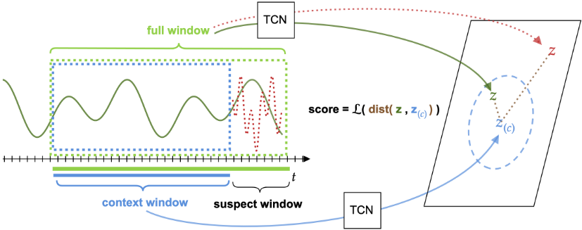
On a given window w ∈ WL(X), we identify a partition of two subsequent segments, w = (w(c) , w(s) ), with lengths C and S (typically C ≫ S), which we call the context window and the suspect window, respectively (see fig. 1 for an illustration).
Our goal is to detect anomalies in the suspect window relative to the local context provided by the context window. We keep a single label y for the windows w, such that y = 1 if any timestep in its suspect segment contains an anomaly, and y = 0 otherwise. In this way, the datasets for training and evaluation are formed by pairs of windows and their labels: D = {(wi, yi)}w∈WL(X )
For our model, we use a neural network encoder ϕ : RT×D → RE to map D-dimensional time series of length T (possibly variable) into fixed-size vector representations. We use a CNN with exponentially dilated causal convolutions [van den Oord et al., 2016], and in particular, the TCN architecture [Franceschi et al., 2019] with adaptive maxpooling along the time dimension.
Let us denote as z = ϕ(w) and z(c) = ϕ(w(c) ) the vector representations of a window w ∈ WL(X) and its context segment w(c) . Intuitively, we want to train ϕ(·) in such a way that representations z and z(c) are pulled together if no anomaly is present in the suspect window, and pushed apart otherwise.
3.2 Contextual Hypersphere Loss
We propose a contrastive loss function, which can be interpreted as a contextual version of the Hypersphere Classifier loss (eq. (1)).
Consider a distance-like function dist(·, ·) : RE ×RE → R+ measuring similarity between two vector representations; and consider a scoring function ℓ : R → [0, 1] mapping distances to pseudo-probabilistic scores in the unit interval.
Our contextual hyperphere loss is defined as:
Note that this is the HSC loss, with the difference that the center of the hypersphere is chosen dynamically for each instance as the representation of the context.
In our experiments, we use the Euclidean distance dist(x, z) = ∥x- z∥2 and a radial basis function ℓ(z) := exp(-z2 ), to create a spherical decision boundary, resulting in the loss function
3.3 Data Augmentation
We introduce a collection of data augmentation methods that inject synthetic anomalies. These data augmentation methods explicitly do not attempt to characterise the full data distribution of anomalies, which would be infeasible. Rather, we combine effective generic heuristics that work well for detecting common types of out-of-distribution examples.
Contextual Outlier Exposure (COE) Motivated by the success of Outlier Exposure for out-of-distribution detection [Hendrycks et al., 2019], we propose a simple taskagnostic method to create contextual out-of-distribution examples. Given a time series window w = (w(c) ,w(s) ), we induce anomalies into the suspect segment, w(s) , by replacing a chunk of its values with values taken from another time series. The replaced values in w(s) will most likely break the temporal relation with their neighboring context, therefore creating an out of distribution example. In our implementation, we apply COE at training time by selecting random examples in a minibatch and permuting a random length of their suspect windows. In multivariate time series, as anomalies do not have to happen in all dimensions, we randomly select a subset of the dimensions in which the windows are swapped.
Anomaly Injection We propose to inject Point Outliers (po) in the time series using a simple method: at a set of randomly selected time points we add (or subtract) a spike to the time series. The spike is proportional to the inter-quartile range of the points surrounding the spike location. Like for COE, in multivariate time series we simply select a random subset of dimensions on which we add the spike. These simple point outliers serve the same purpose as COE: create clear labeled abnormal points to help the learning of the hypersphere. In addition to these, in some practical applications, it is possible to identify general characteristics of anomalies that should be detected. Some widely-known anomalous patterns include: sudden changes in the location or scale of the series (change-points); interruption of seasonality, etc. We have used this approach in our practical application and the domain knowledge allowed to improve the detection performance. As they require and domain knowledge it would be unfair to compare our method when incorporating these; therefore, in the results table we only use the point outliers described above.
WindowMixup If we do not have access to training labels and know little about the relevant anomalies, we mainly rely on COE and po, which may result in significantly missmatch between injected and true anomalies. To improve generalization of our model in this case, we propose to create linear combinations of training examples and their labels inspired by the MIXUP procedure [Zhang et al., 2018]. The MIXUP data augmentation technique was proposed in the context of computer vision and creates more variety in training examples, but more importantly, the soft labels result in smoother decision functions that generalize better. MIXUP is suited for time series applications: convex combinations of time series most often result in realistic and plausible new time series. We show that MIXUP can improve generalization of our model even in cases with a large mismatch between injected and true anomalies.
We include illustrations of these techniques in the extended version of this article 1 .
3.4 NCAD Training
We combine the elements described above and train the encoder by minimizing the contextual hypersphere loss using Stochastic Gradient Descent (SGD).
We start with a raw dataset of time series and their labels (X, Y) = {(x(i) 1:Ti , y(i) 1:Ti )}i=1,...,N . A first augmentation 3 is applied to the series before spliting into windows, yielding (X ′ , Y ′ ) = anomalize((X, Y)). We then define the training dataset by splitting the original and augmented data into windows Daug = {(wi, yi)}wi∈WL(X∪X ′ ) (see section 3.1).
Mini-batches B = {(wi, yi)}i=1,...,batch size are formed by taking random subsets of windows from the training dataset:
3 We inject po during the first augmentation.
B ⊂ Daug . We apply a second stage of data augmentation 4 here by introducing synthetic anomalies on the batches, yielding B′ = anomalize(B).
The score function minimized during training sums the contextual loss function L from eq. (2) over examples in the original and augmented batches:
where θ parametrizes the neural encoder ϕθ(·).
Rolling predictions Once the model is trained, we can apply it to the raw time series in a rolling fashion, possibly defining a stride parameter. Each time step may be part of multiple windows at test time (if the stride is smaller than the suspect window length), obtaining multiple anomaly scores, which can be aggregated by averaging. Such rolling scheme have the advantage of generating anomaly scores with lower latency.
4 Experiments
In this section, we compare the performance of our approach with alternative methods on public benchmark datasets, and exploring the model behavior under different data settings, demonstrating its effectiveness from the unsupervised to the supervised setting. Further details on the experiments are included in the extended version of the article 1 .
4.1 Benchmark Datasets
We benchmark our method to others on five datasets, spanning the univariate, multi-variate, supervised and unsupervised settings.
For the multivariate setting, we use: Soil Moisture Active Passive satellite (SMAP) and Mars Science Laboratory rover (MSL), two datasets published by NASA [Hundman et al., 2018], with 55 and 27 series respectively (lengths of the time series vary from 300 to 8500 observations); and Server Machine Dataset (SMD), a 5 weeks long dataset with 28 38-dimensional time series each collected from a different machine in large internet companies [Su et al., 2019]. These three datasets each have a pre-defined train/test split, where anomalies in the test set are labeled, while the training set contains unlabeled anomalies.
For the univariate setting, we use: YAHOO, a dataset by [Yahoo! Labs, 2015] consisting of 367 real and synthetic time series. And KPI, univariate dataset released in the AIOPS data competition by [Tsinghua Netman Lab, 2018]. It consists of KPI curves from different internet companies in 1 minute interval. 5 For both, following [Ren et al., 2019], we use the last 50% of the time points of each of the time series as test set and split the rest in 30% training and 20% validation set.
4 We use COE and MIXUP during the batch augmentation.
5 While we share many of the concerns expressed by [Wu and Keogh, 2020] about the lack of quality benchmark datasets for time series anomaly detection, we use these commonly-used benchmark datasets here for lack of better alternatives and to enable direct comparison of our approach to competing methods.
| Model | YAHOO (un.) | KPI (un.) | KPI (sup.) | SMAP | MSL | SMD |
|---|---|---|---|---|---|---|
| OC-SVM [Sch¨olkopf et al., 1999] | 4.75 | 5.06 | - | 67.78 | 18.98 | 8.01 |
| Isolation Forest [Liu et al., 2008] | 19.08 | 6.61 | - | 67.78 | 19.21 | 8.77 |
| LOF [Breunig et al., 2000] | 19.08 | 10.56 | - | 70.80 | 39.08 | 36.44 |
| Baseline 1 [Kim et al., 2022] | 20.11 ±2.42 | 68.67 ±0.94 | - | 96.1 | 93.1 | 80.4 |
| SPOT [Siffer et al., 2017] | 33.8 | 21.7 | - | - | - | - |
| DSPOT [Siffer et al., 2017] | 31.6 | 52.1 | - | - | - | - |
| DONUT [Xu et al., 2018] | 2.6 | 34.7 | - | - | - | - |
| SR [Ren et al., 2019] | 56.3 | 62.2 | - | - | - | - |
| SR-CNN [Ren et al., 2019] | 65.2 | 77.1 | - | - | - | - |
| SR+DNN [Ren et al., 2019] | - | - | 81.1 | - | - | - |
| AnoGAN [Schlegl et al., 2017] | - | - | - | 74.59 | 86.39 | - |
| DeepSVDD [Ruff et al., 2018] | - | - | - | 71.71 | 88.12 | - |
| DAGMM [Zong et al., 2018] | - | - | - | 82.04 | 86.08 | 72.3 |
| LSTM-VAE [Park et al., 2018] | - | - | - | 75.73 | 73.79 | 80.8 |
| MSCRED [Zhang et al., 2019] | - | - | - | 77.45 | 85.97 | 38.9 |
| MTAD-GAT [Zhao et al., 2020] | - | - | - | 90.13 | 90.84 | - |
| OmniAnomaly [Su et al., 2019] | - | - | - | 84.34 | 89.89 | 94.4 |
| THOC [Shen et al., 2020] | - | - | - | 95.18 | 93.67 | 54.1 |
| USAD [Audibert et al., 2020] | - | - | - | 81.86 | 91.09 | 93.82 |
| NCAD w/ COE, po , mixup | 81.16 ±1.43 | 76.64 ±0.89 | 83.30 ±0.87 | 94.45 ±0.68 | 95.60 ±0.59 | 80.16 ±0.69 |
4.2 Evaluation Setup
Measuring the performance of time series anomaly detection methods in a universal way is challenging, as different applications often require different trade-offs between sensitivity, specificity, and temporal localization. To account for this, various measures that improve upon simple pointwise classification metrics have been proposed, e.g. the flexible segment-based score proposed by [Tatbul et al., 2018] or the score used in the Numenta anomaly benchmark [Lavin and Ahmad, 2015]. To make our results directly comparable, we follow the procedure proposed by [Xu et al., 2018] (and subsequently used in other work [Su et al., 2019; Ren et al., 2019; Shen et al., 2020]), which offers a practical compromise: point-wise scores are used, but the predicted labels are expanded to mark an entire true anomalous segment as detected correctly if at least one time point was detected by the model. 6 Shortcomings of this evaluation protocol have been uncovered by [Kim et al., 2022]: if the dataset has many long segments labeled as anomalous (as e.g. in the SWaT and SMAP datasets), then the correction allows high F1 scores to be achieved even based on weak (or even random) anomaly scores. However, as they also point out, this is less of a problem when anomalies are very short as in KPI and YAHOO. To emphasize this point we include the F1 scores for the baseline that they proposed, which performs significantly worse on the data sets with short anomaly segments. While in practice a detection threshold would have to be chosen on a validation set or through user input, we align our experimental protocol with this body of prior work and report optimistic F1 scores computed by choosing the best threshold on the test set. For each dataset, a single best threshold is chosen and used on all the time series of the test set. 7
6 We use the implementation by [Su et al., 2019].
Hyperparameters were chosen using the validation set for YAHOO and KPI, and a standard setting is inferred for the other datasets (see extended article for details 1 ). We use short suspect windows because we are interested in the harder problem of streaming anomaly detection where it is important to detect anomalous points early. Further, we run the model 10 times on each of the benchmark datasets and report mean and standard deviation. We provide scripts to reproduce the results on the benchmark datasets shown below.
Comparison partners Beyond several deep state of the art methods, we compare to a set of classical shallow anomaly detection methods on fixed time series windows: OC-SVM [Sch¨olkopf et al., 1999], Isolation Forest [Liu et al., 2008], and LOF [Breunig et al., 2000]. In addition, we compare to a non-deep probabilistic method using Gaussian processes [Bock et al., 2022]. We also include the baseline 1 of [Kim et al., 2022], for which the anomaly score of each point is sampled from a uniform distribution.
4.3 Benchmark Results
Table 1 shows the performance of our NCAD approach compared to the state-of-the-art methods proposed for the different datasets and settings, as well as a set of non-time series baselines.
The univariate datasets contain labels for anomalies both on the training and the test set, we evaluate our method on them both in the supervised setting ((sup.)) and the unsupervised setting ((un.)). Our approach significantly outperforms competing approaches on YAHOO, performs similarly to the best unsupervised approach on KPI, and better than the best supervised approach.
7 Note that this is done for all methods, keeping the relative performance of different methods comparable, even if the absolute scores are higher than what can be expected in a practical setting.
| YAHOO | |||
|---|---|---|---|
| MODEL | F1 | PREC | REC |
| U-NET-RAW | 40.3 | 47.3 | 35.1 |
| U-NET-DE | 62.1 | 65.1 | 59.4 |
| U-NET-DEW | 66.2 | 79.3 | 56.9 |
| U-NET-DEWA | 69.3 | 85.9 | 58.1 |
| NCAD SUPERVISED | 62.11 | 80.44 | 50.59 |
| + MIXUP | 63.08 | 76.70 | 53.57 |
| + PO | 79.92 | 74.96 | 85.57 |
| + COE | 53.66 | 78.84 | 40.67 |
| + COE + MIXUP | 59.85 | 78.89 | 48.21 |
| + PO + COE | 58.36 | 54.89 | 62.30 |
| + PO + COE + MIXUP | 67.32 | 88.38 | 54.36 |
| - CONTEXTUAL | 5.50 | 3.42 | 14.08 |
| - CONTEXTUAL + PO | 67.90 | 64.15 | 72.13 |
| - CONTEXTUAL + COE | 39.53 | 42.56 | 36.90 |
| - CONTEXTUAL + PO + COE | 55.25 | 43.87 | 74.60 |
It is important to note that while other methods are either designed for the supervised or unsupervised setting, our method can be used seamlessly in both settings. For NCAD, in the supervised setting the training labels are used in the loss, whereas in the unsupervised setting only the labels of the simple synthetic anomalies are used for training.
For KPI (sup.) we only compare to a single baseline because the other methods are not developed for the supervised context. The YAHOO-supervised experiments are included in table 2, our approach outperforms the state-of-the-art [Gao et al., 2020] significantly with 79% point-wise F1 score versus 69.3% F1 score for their approach.
On the multivariate datasets, all benchmark methods are designed for unsupervised anomaly detection, and none of the dataset contains training labels. Our method outperforms the state of the art by a reasonable margin on MSL. On SMAP our average score is slightly lower than the best score. On SMD, OmniAnomaly and USAD outperform our approach. We note that these methods train one model for each of the 28 time series, while we train a single global model, which is more representative of a real world scenario.
4.4 Ablation Studies
To better understand the advantage brought by each of the components of our method, we perform an ablation study on the SMAP and MSL datasets, shown in table 3. The first row corresponds to the entire NCAD framework, using contextual hypersphere loss and data augmentation. The rows labeled "- contextual . . . " do not use the contextual hypersphere described in section 3.2, but instead a model trained using the original hypersphere classifier loss on the whole-window representation ϕ(w). First, we see that the contextual hypersphere has a significant impact on performance when no data augmentation is used, increasing performance by 11.81% F1 on SMAP and 43.44% F1 on MSL. By only removing the contextual hypersphere but keeping the data augmentation methods ("- contextual" row), we observe a small performance deterioration with respect to the full model, 1.98% F1 on SMAP and 1.17% F1 on MSL.
| Model | SMAP | MSL |
|---|---|---|
| NCAD w/ COE, po, mixup | 94.45 ± 0.7 | 95.60 ± 0.7 |
| - po | 94.28 ± 0.4 | 94.73 ± 0.3 |
| - COE | 88.59 ± 1.8 | 94.66 ± 0.2 |
| - mixup | 92.69 ± 1.1 | 95.59 ± 0.01 |
| - mixup - po | 94.4 ± 0.4 | 94.12 ± 0.8 |
| - mixup - COE | 86.86 ± 0.7 | 91.7 ± 2.6 |
| - COE - po | 60.48 ± 9.7 | 42.02 ± 6.3 |
| - mixup - COE - po | 66.9 ± 2.0 | 79.47 ± 9.4 |
| - contextual | 92.47 ± 0.5 | 94.43 ± 0.1 |
| - contextual - COE | 91.86 ± 1.0 | 88.29 ± 0.4 |
| - contextual - po | 93.39 ± 0.6 | 90.68 ± 0.7 |
| - contextual - mixup | 94.37 ± 0.2 | 95.07 ± 0.1 |
| - contextual - mixup - po | 93.24 ± 0.3 | 90.89 ± 0.5 |
| - contextual - mixup - COE | 89.88 ± 2.5 | 87.26 ± 4.2 |
| - contextual - COE - po | 54.95 ± 2.62 | 32.0 ± 0.2 |
| - context. - COE - mixup - po | 55.09 ± 1.0 | 36.03 ± 3.0 |
We also see that each of the data augmentation techniques improves the performance further.
Further ablation results on the supervised Yahoo dataset can are shown in table 2. Using only the true labels but no data augmentation (NCAD SUPERVISED), our approach significantly outperforms U-NET-RAW, and performs on-par with U-NET-DE, without relying on time series decomposition and using an arguably much simpler architecture.
When we use the po data augmentation, our approach outperforms the full U-NET-DEWA by a large margin, hinting at the possibility that addressing the class imbalance problem by creating artificial anomalies is more effective than using their strategy of loss weighting while keeping the labels intact.
In the supervised setting, injecting the generic COE anomalies (either individually or in combination with po) hurts performance, presumably by steering the model away from the specific kind of anomalies that are labeled as anomalous in this data set. On the other hand, adding MIXUP generally improves performance. The contrastive loss is crucial for good performance, as shown by the rows labeled - CONTRASTIVE, where it is replaced with a standard softmax classifier.
4.5 Scaling FromUnsupervised to Supervised
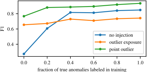
To investigate how the performance of our approach changes as we scale from unsupervised, to semi-supervised, to fully supervised, we measure the performance of our approach as a function of the amount of ground truth labels on the YAHOO dataset, shown in fig. 2.
Firstly, we observe that the performance increases steadily with the amount of true anomaly labels, as desired. Secondly, by using synthetic anomalies (either po or COE), we can significantly boost the performance in the regime when no or only few labels are available. Finally, by using an injection technique that is well-aligned with the desired type of anomalies (po in this case, as YAHOO contains a large number of single-point outliers), one can significantly improve performance over relying solely on the labeled data, this is explained by the very high class imbalance in anomaly detection. The flipside is, of course, that injecting anomalies that may be significantly different from the desired anomalies (COE in this case) can ultimately hurt when enough labeled examples are available.
| Model | SMAP 1st dimension |
|---|---|
| NCAD w/ COE, po, mixup | 93.38 |
| NCAD w/ COE, po, mixup, + domain informed injections | 96.48 |
4.6 Using Specialized Anomaly InjectionMethods
In many practical applications one may have access to some domain knowledge about the type of anomalies that are to be detected, our method allows to incorporate this easily. While in all our benchmarks we rely on completely generic anomalies for injection (COE and po), a by-product of our methodology is that the model can be guided towards detecting the desired class of anomalies by designing anomaly injection methods that mimic the true anomalies. Designing such methods is often simple compared to finding enough examples of true anomalies as they are rare.
Table 4 demonstrates the effectiveness of this approach: The first dimension of the SMAP dataset contains slow slopes that are labeled as anomalous in the dataset. These are harder to detect for our model when only using COE and po because these cannot create similar behavior. We can design a simple anomaly injection that injects slopes to randomly selected regions and labels them as anomalous. Training NCAD with these slopes gives a model that achieves a much better score.
This approach can be effective in applications where anomalies are subtle and closer to the normal data, and where some prior knowledge is available about the kind of anomalies that are to be detected. However one may not have this prior knowledge or the resources required to create these injections. This is a limitation of this technique which prevents it from being generally applicable. This is the reason why we did not use in for the comparison to the other methods.
4.7 Generalization From Injected Anomalies
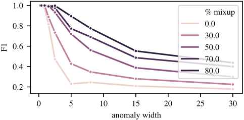
Artificial anomalies will always differ from the true anomalies to some extent, be it the ones created by COE, po, or more complex methods. This requires the model to generalize from imperfect training examples to true anomalies. By design, the hypersphere formulation can help to bridge this generalization gap, and we use MIXUP further improve the generalization capabilities of the model.
Figure 3 shows the results of an experiment exploring one aspect of this generalization ability for NCAD. The model is trained with injected single-point outliers, and we measure the detection performance for anomalies of longer width. For this experiment we use a synthetic base data set containing simple sinusoid time series with Gaussian noise. We create multiple datasets from this base dataset adding true anomalies of varying width by convolving spike anomalies with Gaussian filters of different widths. For training, regardless of the shape of the true anomalies, we use po and train models using different MIXUP rates, i.e. fraction of training examples with MIXUP applied. We observe that MIXUP helps the model to generalize in this setting: the higher the MIXUP rate, the better the model generalizes to anomalies that differ from the injected examples, achieving higher F1 scores.
5 Conclusion
We present NCAD, a methodology for anomaly detection in time series that achieves state-of-the-art performance in a broad range of settings, including both the univariate and multivariate cases, as well as across the unsupervised, semisupervised, and supervised anomaly detection regimes. We demonstrate that combining expressive neural representation for time series with data augmentation techniques can outperform traditional approaches such as predictive models or methods based on reconstruction error.
@inproceedings{ijcai2022p394,
  title     = {Neural Contextual Anomaly Detection for Time Series},
  author    = {Carmona, Chris U. and Aubet, François-Xavier and Flunkert, Valentin and Gasthaus, Jan},
  booktitle = {Proceedings of the Thirty-First International Joint Conference on
               Artificial Intelligence, {IJCAI-22}},
  publisher = {International Joint Conferences on Artificial Intelligence Organization},
  editor    = {Luc De Raedt},
  pages     = {2843--2851},
  year      = {2022},
  month     = {7},
  note      = {Main Track},
  doi       = {10.24963/ijcai.2022/394},
  url       = {https://doi.org/10.24963/ijcai.2022/394},
}
TY - CPAPER TI - Neural Contextual Anomaly Detection for Time Series AU - Carmona, Chris U. AU - Aubet, François-Xavier AU - Flunkert, Valentin AU - Gasthaus, Jan T2 - Proceedings of the Thirty-First International Joint Conference on Artificial Intelligence, IJCAI-22 PB - International Joint Conferences on Artificial Intelligence Organization PY - 2022 SP - 2843 EP - 2851 DO - 10.24963/ijcai.2022/394 UR - https://doi.org/10.24963/ijcai.2022/394 ER -Copied
Machine-readable versions of this paper, for tools and AI agents:





