
Rethinking the Promotion Brought by Contrastive Learning to Semi-Supervised Node Classification
Proceedings of the Thirty-First International Joint Conference on Artificial Intelligence. Main Track. Pages 2852-2858.
https://doi.org/10.24963/ijcai.2022/395
Keywords
- Machine Learning: Sequence and Graph Learning
- Machine Learning: Semi-Supervised Learning
- Data Mining: Mining Graphs
Abstract
Graph Contrastive Learning (GCL) has proven highly effective in promoting the performance of Semi-Supervised Node Classification (SSNC). However, existing GCL methods are generally transferred from other fields like CV or NLP, whose underlying working mechanism remains underexplored. In this work, we first deeply probe the working mechanism of GCL in SSNC, and find that the promotion brought by GCL is severely unevenly distributed: the improvement mainly comes from subgraphs with less annotated information, which is fundamentally different from contrastive learning in other fields. However, existing GCL methods generally ignore this uneven distribution of annotated information and apply GCL evenly to the whole graph. To remedy this issue and further improve GCL in SSNC, we propose the Topology InFormation gain-Aware Graph Contrastive Learning (TIFA-GCL) framework that considers the annotated information distribution across graph in GCL. Extensive experiments on six benchmark graph datasets, including the enormous OGB-Products graph, show that TIFA-GCL can bring a larger improvement than existing GCL methods in both transductive and inductive settings. Further experiments demonstrate the generalizability and interpretability of TIFA-GCL.
- [Bai et al., 2021] S. Bai, F. Zhang, and P. H. Torr. Hypergraph Con- volution and Hypergraph Attention. Pattern Recognit., 2021.
- [Bianchi et al., 2019] F. M Bianchi, D. Grattarola, L. Livi, and C. Alippi. Graph Neural Networks with Convolutional Arma Fil- ters. arXiv: 1901.01343, 2019.
- [Buchnik and Cohen, 2018] Eliav Buchnik and Edith Cohen. Boot- strapped Graph Diffusions: Exposing the Power of Nonlinearity. Proc. ACM Meas. Anal. Comput. Syst., 2(1):10:1-10:19, 2018.
- [Chen et al., 2021] S. Chen, Z. W., X. Z., X. Z., and D. P. Probing Negative Sampling Strategies to Learn Graph Representations via Unsupervised Contrastive Learning. arXiv: 2104.06317, 2021.
- [Defferrard et al., 2016] Michaël Defferrard, Xavier Bresson, and Pierre Vandergheynst. Convolutional Neural Networks on Graphs with Fast Localized Spectral Filtering. In NeurIPS, 2016.
- [Feng et al., 2020] Wenzheng Feng, Jie Zhang, Yuxiao Dong, Yu Han, Huanbo Luan, Qian Xu, Qiang Yang, Evgeny Khar- lamov, and Jie Tang. Graph random neural networks for semi- supervised learning on graphs. In NeurIPS, 2020.
- [Hamilton et al., 2017] W. L. Hamilton, Z. Ying, and J. L. Inductive Representation Learning on Large Graphs. In NeurIPS, 2017.
- [Hassani and Khasahmadi, 2020] Kaveh Hassani and Amir Hosein Khasahmadi. Contrastive Multi-View Representation Learning on Graphs. In ICML, 2020.
- [He et al., 2020] Kaiming He, Haoqi Fan, Yuxin Wu, Saining Xie, and Ross Girshick. Momentum Contrast for Unsupervised Visual Representation Learning. In CVPR, 2020.
- [Hu et al., 2020] Weihua Hu, Matthias Fey, Marinka Zitnik, Yux- iao Dong, Hongyu Ren, Bowen Liu, Michele Catasta, and Jure Leskovec. Open Graph Benchmark: Datasets for Machine Learn- ing on Graphs. In NeurIPS, 2020.
- [Jovanovic et al., 2021] Nikola Jovanovic, Zhao Meng, Lukas Faber, and Roger Wattenhofer. Towards Robust Graph Con- trastive Learning. arXiv: 2102.13085, 2021.
- [Kefato and Girdzijauskas, 2021] Zekarias T. Kefato and Sarunas Girdzijauskas. Self-supervised Graph Neural Networks without Explicit Negative Sampling. arXiv: 2103.14958, 2021.
- [Kipf and W., 2017] T. N. Kipf and M. W. Semi-supervised Classi- fication with Graph Convolutional Networks. In ICLR, 2017.
- [Morris et al., 2019] Christopher Morris, Martin Ritzert, Matthias Fey, William L Hamilton, Jan Eric Lenssen, Gaurav Rattan, and Martin Grohe. Weisfeiler and Leman go Neural: Higher-order Graph Neural Networks. In AAAI, 2019.
- [Qiu et al., 2020] Jiezhong Qiu, Qibin Chen, Yuxiao Dong, Jing Zhang, Hongxia Yang, Ming Ding, Kuansan Wang, and Jie Tang. GCC: Graph Contrastive Coding for Graph Neural Network Pre- Training. In KDD, 2020.
- [Qu et al., 2021] Y. Qu, D. S., Y. S., S. S., W. C., and J. H. CoDA: Contrast-enhanced and Diversity-promoting Data Augmentation for Natural Language Understanding. In ICLR, 2021.
- [Robinson et al., 2021] Joshua David Robinson, Ching-Yao Chuang, Suvrit Sra, and Stefanie Jegelka. Contrastive Learning with Hard Negative Samples. In ICLR, 2021.
- [Schroff et al., 2015] Florian Schroff, Dmitry Kalenichenko, and James Philbin. Facenet: A Unified Embedding for Face Recog- nition and Clustering. In CVPR, 2015.
- [Sen et al., 2008] Prithviraj Sen, Galileo Namata, Mustafa Bilgic, Lise Getoor, Brian Galligher, and Tina Eliassi-Rad. Collective Classification in Network Data. AI magazine, 29(3):93-93, 2008.
- [Shchur et al., 2018] Oleksandr Shchur, Maximilian Mumme, Aleksandar Bojchevski, and Stephan Günnemann. Pitfalls of Graph Neural Network Evaluation. arXiv: 1811.05868, 2018.
- [Sohn et al., 2020] K. Sohn, D. Berthelot, C. Li, Z. Zhang, N. Car- lini, E. D. Cubuk, A. Kurakin, H. Zhang, and C. Raffel. Fix- match: Simplifying Semi-supervised Learning with Consistency and Confidence. In NeurIPS, 2020.
- [Veličković et al., 2018] Petar Veličković, Guillem Cucurull, Aran- txa Casanova, Adriana Romero, Pietro Lio, and Yoshua Bengio. Graph Attention Networks. In ICLR, 2018.
- [Velickovic et al., 2019] Petar Velickovic, William Fedus, William L. Hamilton, Pietro Liò, Yoshua Bengio, and R. Devon Hjelm. Deep Graph Infomax. In ICLR, 2019.
- [Verma et al., 2018] Nitika Verma, Edmond Boyer, and Jakob Ver- beek. Feastnet: Feature-steered Graph Convolutions for 3d Shape Analysis. In CVPR, 2018.
- [Verma et al., 2019] Vikas Verma, Meng Qu, Alex Lamb, Yoshua Bengio, Juho Kannala, and Jian Tang. GraphMix: Regularized Training of Graph Neural Networks for Semi-Supervised Learn- ing. arXiv: 1909.11715, 2019.
- [Wan et al., 2021] S. Wan, S. Pan, J. Yang, and C. Gong. Con- trastive and Generative Graph Convolutional Networks for Graph-based Semi-Supervised Learning. In AAAI, 2021.
- [Wang and Leskovec, 2020] Hongwei Wang and Jure Leskovec. Unifying Graph Convolutional Neural Networks and Label Prop- agation. arXiv: 2002.06755, 2020.
- [Wang and Liu, 2021] Chenguang Wang and Ziwen Liu. Graph Representation Learning by Ensemble Aggregating Subgraphs via Mutual Information Maximization. arXiv: 2103.13125, 2021.
- [Wang et al., 2020] Yiwei Wang, Wei Wang, Yuxuan Liang, Yujun Cai, Juncheng Liu, and Bryan Hooi. NodeAug: Semi-Supervised Node Classification with Data Augmentation. In KDD, 2020.
- [Xie et al., 2021] Qizhe Xie, Zihang Dai, Eduard H. Hovy, Thang Luong, and Quoc Le. Unsupervised Data Augmentation for Con- sistency Training. In NeurIPS, 2021.
- [Yang et al., 2016] Zhilin Yang, William W Cohen, and Ruslan Salakhutdinov. Revisiting Semi-supervised Learning with Graph Embeddings. In ICML, 2016.
- [Yang et al., 2020] Zhen Yang, Ming Ding, Chang Zhou, Hongxia Yang, Jingren Zhou, and Jie Tang. Understanding Negative Sam- pling in Graph Representation Learning. In KDD, 2020.
- [You et al., 2020] Yuning You, Tianlong Chen, Yongduo Sui, Ting Chen, Zhangyang Wang, and Yang Shen. Graph Contrastive Learning with Augmentations. In NeurIPS, 2020.
- [Zeng et al., 2020] Hanqing Zeng, Hongkuan Zhou, Ajitesh Srivas- tava, Rajgopal Kannan, and Viktor K. Prasanna. GraphSAINT: Graph Sampling Based Inductive Learning Method. In ICLR, 2020.
- [Zhu et al., 2020] Yanqiao Zhu, Yichen Xu, Feng Yu, Qiang Liu, Shu Wu, and Liang Wang. Deep Graph Contrastive Representa- tion Learning. arXiv: 2006.04131, 2020.
- [Zhu et al., 2021] Yanqiao Zhu, Yichen Xu, Feng Yu, Qiang Liu, Shu Wu, and Liang Wang. Graph Contrastive Learning with Adaptive Augmentation. In WWW, 2021.
References were extracted automatically from the PDF and may contain errors.
Full text extracted automatically from the PDF; figures, tables and equations may differ. The PDF is the version of record.
1 Introduction
Graph 1 Neural Networks (GNNs) can effectively utilize the relation of nodes from graph and have shown powerful modeling capabilities [Yang et al., 2016] in Semi-Supervised Node Classification (SSNC). Nevertheless, vanilla GNN training [Kipf and W., 2017] accesses the training signal mainly from the limited labeled nodes and pays little attention to the massive information contained in the unlabeled nodes. To fix this, recent studies [Hassani and Khasahmadi, 2020; Zhu et al., 2020; Zhu et al., 2021; You et al., 2020; Wan et al., 2021; Feng et al., 2020] introduce Contrastive Learning (CL) into graph scene to leverage the information of the unlabeled nodes and have achieved promising performance.
1 Part of the work was done while Peng Li was working at Tencent.
Though successful, the working mechanism of Graph Contrastive Learning (GCL) in SSNC remains under-explored because the graph scene is fundamentally different from the other scenes like image or text. The samples are connected by complex edges and the task-related annotated information are propagated from the labeled nodes to the unlabeled nodes through graph topology, which results in an imbalanced distribution of the annotated information distribution across the graph. Therefore, how this imbalanced distribution can affect GCL running and why CL works in the SSNC task have become essential research questions in this field.
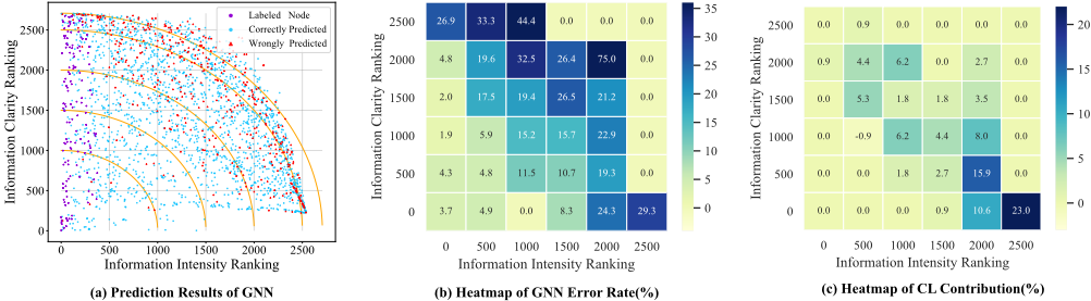
In this work, we first investigate how the annotated information distribution affects the GCL effect. We employ the well-known Label Propagation [Buchnik and Cohen, 2018] method to measure the annotated information distribution. We find that the promotion of GCL mainly comes from those nodes with less annotated information. Specifically, in Figure 1, we notice that GNN's inference ability decays radially outward in the annotated information intensity-clarity coordinate system, while GCL's effect, in contrast, increases radially outward. However, existing GCL methods overlook this phenomena and apply CL to the whole graph evenly.
Motivated by our findings, we propose the Topology InFormation gain-Aware Graph Contrastive Learning (TIFA-GCL) framework to enhance the GCL methods from two aspects: (1) from the global view of the whole graph, we enhance the GCL effect on nodes that receive less annotated information from the information source (labeled nodes), by devising novel self-adaptive graph corruption and CL loss weight schedule mechanisms; and (2) from the local view of each node, we observe that nodes with similar annotated information distribution are more likely to share the same class label, based on which we promote the contrastive pair sampling and subgraph sampling strategies. Extensive experiments on six benchmark datasets, including the enormous OGB-Products graph [Hu et al., 2020], have shown that our method can bring more significant improvements to GNN training compared to existing GCL methods in both transductive and inductive setting. Further investigations are provided to answer several important research questions of our work.
2 ACloser Look at GCL in Semi-Supervised Node Classification
Owing to the success of GCL in SSNC, we attempt to probe its working mechanism in this section. Since nodes' received annotated information has a crucial impact on GNN's inference performance, we first introduce a measurement for the node's received annotated information from the labeled nodes along graph topology, and then investigate how the annotated information will affect the performance of GCL from the perspectives of information intensity and clarity.
2.1 Task Formalization
We follow the benchmark setting [Kipf and W., 2017; Yang et al., 2016; Hamilton et al., 2017] to discuss the working mechanism of GCL in the semi-supervised node classification task. Formally, given an undirected graph G = (V, E), where V is the node set with an embedding matrix X ∈ Rn×h (n = |V| , h is the feature dimension size) and E is the edge set represented by an adjacency matrix A ∈ Rn×n , the node classification task aims to learn a classifier F to predict the class label y for each node. We denote the labeled and unlabeled node sets as L and U, respectively.
2.2 Measuring the Annotated Information from the Labeled Nodes
In this work, we employ the Label Propagation [Buchnik and Cohen, 2018] (LP) algorithm to measure the annotated information distribution among the graph nodes that have complex connections with graph edges. LP is a very popular method for SSNC based on the message-passing mechanism: the labels are propagated from the labeled nodes to the unlabeled nodes through graph edges. We adopt LP to measure the annotated information distribution for two reasons: (1) LP focuses on the graph topology, which can reflect the annotated information clearly; (2) LP shares the same mechanism (message-passing) with many GNN models [Wang and Leskovec, 2020], so the conclusions of it can be transferred to general GNN models like GCN [Kipf and W., 2017] and GraphSAGE [Hamilton et al., 2017]. The LP method can be formulated as:
I is the identity matrix; α ∈ (0, 1] represents the random walk restart probability. A′ = AD-1 and D is the node degree matrix. Z ∈ Rn∗k is the convergence result of LP; Zi,j indicates the probability that the the i-th node is belong to the j-th class and we regard it as the influence received by the i-th node from the j-th class's labeled nodes; Z0 in the initial label matrix where labeled nodes are represented by one-hot vectors and unlabeled nodes are filled with zero. In practice, we take a updated version Z∗ to consider the category preference of nodes (shown in Appendix A1 2 ).
2.3 Probing the Mechanism of GCL
In this part, we analyze the working mechanism of GCL with the help of LP. Ideally, the received information for each node should be concentrated on one category, which means that the annotated information is strong and clear. So we regard the maximum item of vector Z∗ i,: to be the information intensity and the gap to the others as the information clarity for node i:
where max(·) returns the max value of the input vector. With QIntensity and QClarity , we conduct an analysis experiment on the benchmark CORA [Sen et al., 2008] dataset trained by GCN [Kipf and W., 2017] in Figure 1. We plot the prediction results in the QIntensity ×QClarity rectangular coordinate system in Figure 1 (a). Figure 1 (b) shows the error rates for different grids from Figure 1 (a). From Figure 1 (a)(b), we can find that, the graph nodes in SSNC are distributed in a fan shape, which means that there is no nodes with low QIntensity and low QClarity at the same time. Moreover, we notice that the GNN's inference ability has the characteristic of radial decay 3 : GNN can predict accurately for nodes around the origin of coordinate, which have both high QIntensity and high QClarity ; however, the GNN inference ability decays radially outward from the origin of coordinate, where nodes receive more noise (information from other classes' labeled nodes) and less helpful information. Figure 1 (c) displays the contribution of GCL effect (the improvement to GNN) among all the grids from Figure 1 (a). We can find that just in contrary to GNN's inference ability, GCL's effect has the characteristic of radial increase: the farther the sector away from the origin of the coordinate, the greater the improvement brought by GCL. Besides, comparing to nodes with high QIntensity and lowQClarity (upper left in plot), GCL enhances GNN's learning ability for nodes with low QIntensity and high QClarity (low right in plot) more effectively. We analyze the reason lies in that nodes with high QIntensity and low QClarity are strongly influenced by graph learning and can be hardly corrected by CL.
2 Appendix Link: https://arxiv.org/abs/2012.07437
Inspired by the fan-shaped distribution of graph nodes and the radical decay phenomenon in GNN, we quantitatively measure each node's Topology Information Gain (short as TIG, indicating the quality of nodes' received annotated information in this work) by jointly considering the node information intensity and clarity. The TIG value Ti for the i-th node is calculated in the following equation:
where λ is the weight of information clarity. The GCL effect across TIG bins is shown in Appendix A3. We summary that: The promotion of GCL mainly comes from nodes with less annotated information in the SSNC task.
3 Methodology
In this section, we first introduce the whole framework of our method in Section 3.1, and then introduce how we modify the CL loss accumulation (Section 3.2), graph perturbation (Section 3.3) and contrastive pair sampling (Section 3.4) to consider the annotated information distribution and promote the CL effect. Moreover, a novel subgraph sampling (shown in Appendix B2) method called SAINT-TIFA is proposed for the inductive setting.
3.1 TIFA-GCL Framework
Generally, in semi-supervised GCL, the training objective consists of two parts: the supervised cross-entropy loss and the unsupervised contrastive loss. Given a GNN encoder F (e.g., GCN), the supervised cross-entropy loss LCE is calculated on the labeled set L:
3 Similar phenomenon is found in other datasets (Appendix A2).
where gi is the GNN output for node i; yi is the gold label in one-hot embedding; θ is the parameters of F. Apart from LCE, the contrastive loss in TIFA-GCL contains two parts: a self-consistency loss and a pair-wise loss with positive and negative pairs. The self-consistency loss is calculated in the following equation:
where KL(·, ·) is the Kullback-Leibler divergence function; the augmented node embedding matrix Xp and the adjacency matrix Ap are generated by the TIFA-graph perturbation which is detailed in Section 3.3. Following [Xie et al., 2021] and [Wang et al., 2020], ˜ θ is a fixed copy of the current parameter θ and the gradient is not propagated through ˜ θ. Similarly, the contrastive loss with positive and negative pairs is computed as:
where Pi and Ni are the positive and negative pairs for the i-th node generated by our TIFA-contrastive pair sampling strategy introduced in Section 3.4, µ1 is a hyper-parameters to control the weight of GCL loss of negative pairs comparing to positive pairs. Then the complete unsupervised loss on node i is calculated via:
where µ2 controls the weight of Lip relative to Lis .
3.2 TIFA-Contrastive Loss Weight Schedule
Different from all the existing GCL studies [Zhu et al., 2020; Wan et al., 2021; Wang et al., 2020; Zhu et al., 2021; Hassani and Khasahmadi, 2020; You et al., 2020; Feng et al., 2020], which accumulate the unsupervised contrastive loss from different nodes directly, we instead propose to adjust the CL loss weight adaptively among different subgraphs according to their TIG. Specifically, we set the CL weight wi of each node differently using a cosine annealing schedule based on the node TIG ranking 4 :
where wmin,wmax are the hyper-parameters indicating the minimum and the maximum values of CL loss, respectively; Rank(Ti) is the ranking order of Ti from the smallest to the largest. Then the final training objective of TIFA-GCL consists of the supervised loss and a weighted-sum of the unsupervised contrastive loss:
4 We also try other schedule methods like linear schedule, piecewise schedule and scheduling based on the absolute TIG value instead of the relative ranking. The experiment results show the cosine method works best.
With this manner, subgraphs receiving less annotated information from graph topology can benefit more from GCL, forming a more adaptive combination of graph representation learning and graph contrastive learning.
3.3 TIFA-Graph Perturbation
Unlike perturbation in images [He et al., 2020; Sohn et al., 2020] where samples can be perturbed independently, graph nodes interact with each other and the disturbance of one node will spread to its adjacent neighbors. Therefore, if we perturb too many nodes or edges in graph, the augmented graph will be too different from the original one and thus weakening the GCL effect. We propose that the limited graph perturbation should be more likely to take place on subgraphs with insufficient information gain from graph learning. Thus, we propose to sample nodes to disturb according to their TIG values: a node will be selected with a higher probability for augmentation when it has a lower TIG value. Comparing to the contrastive loss weight schedule which directly adjusts the CL weight, weighted graph perturbation is a more essential method to enhance GCL effect on nodes with fewer TIG values since graph perturbation is the upstream operation of computing CL target. The details of TIFA-graph perturbation algorithm is shown in Appendix B1.
3.4 TIFA-Contrastive Pair Sampling
Contrastive pair sampling, especially the negative pair sampling, has a crucial impact on CL [Robinson et al., 2021; Yang et al., 2020]. Different from existing works which simply regard all other nodes [Wang et al., 2020; Zhu et al., 2020] or labeled nodes from other class [Wan et al., 2021] as negative samples, we propose to sample contrastive pairs based on the relative distance between nodes.
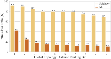
In Figure 2, we observe that nodes with similar annotated information distribution are more likely to share the same class label with each other, and vice versa. Therefore, our measurement for the node relative distance mainly depends on the difference of node LP result, which contains both the global topology information and annotated information. Specifically, we normalize the each node's LP vector and then calculate the KL divergence between nodes as the global topology distance:
where softmax(·) function is adopted to transfer the original LP matrix (Z∗ ) into a probability distribution over all the categories. Besides, we supplement the relative distance measuring from the view of local topology distance and the node embedding distance. For local topology distance Dl i,j , we use the minimum jump hop number as an indicator. For node embedding distance De i,j , we calculate the cosine distance between the nodes in embedding X. The final node relative distance is calculated by the weighted sum of the global/local topology distance and the node embedding distance:
where λ1, λ2 is the weight of the two supplement items; S(·) represents the scale operation to transfer the original value to [0, 1]. Then we construct positive and negative pairs for each node individually. For the i-th node (anchor node), the positive set Pi is composed of the closest nodes with the smallest relative distance; for the negative set Ni, we propose to take the semi-difficult nodes [Schroff et al., 2015] which are neither too far or too close to the anchor node. Given the personally ranked node list Ri sorted by Di from the smallest to the largest (the i-th node itself is excluded), Pi andNi are truncated fromRi, respectively:
where postend is the end index for positive set; negtbeg and negtend are the begin and end indexes for negative set.
4 Experiments
In this section, we first give a brief introduction to the experiment datasets and settings. Followingly, we show the effectiveness of the proposed TIFA-GCL method by comparing with advanced GNN models and other GCL methods in both transductive and inductive settings.
4.1 Datasets and Experimental Settings
We conduct experiments on six widely-used graph datasets, namely paper citations networks [Sen et al., 2008] (CORA,CiteSeer and Pubmed; these three datasets are the mostly-used benchmark networks [Yang et al., 2016; Kipf and W., 2017; Veliˇckovi´c et al., 2018] in the SSNC studies), Amazon Co-purchase networks [Shchur et al., 2018] (Photo and Computers) and the enormous OGB-Products graph [Hu et al., 2020]. More details about the datasets, experiment settings and hyper-parameters can be found in Appendix C.
4.2 Overall Results
The overall results of our proposed methods in transductive and inductive setting are shown in Table 1 and 2, respectively. For the transductive experiments, we set two lines of baselines to verify the effectiveness of our method:(1) Popular GNN models, including GCN [Kipf and W., 2017], GAT [Veliˇckovi´c et al., 2018], GraphSAGE [Hamilton et al., 2017] and GraphMix [Verma et al., 2019]; (2) Existing GCL methods which apply CL to graph uniformly
| Method | CORA | CiteSeer | PubMed | Photo | Comp. |
|---|---|---|---|---|---|
| GCN GAT GraphMix GRACE | 81.0±0.7 79.9±2.1 80.7±1.2 81.5±0.9 | 69.1±0.8 69.6±1.4 67.8±1.4 69.3±0.4 | 76.8±0.8 77.2±1.0 76.3±0.6 78.0±1.3 77.8±1.8 78.4±0.7 | 88.0±1.7 88.7±1.9 87.7±1.2 89.5±1.7 89.3±1.3 89.7±1.8 | 80.7±0.7 |
| 77.9±2.1 | |||||
| GraphSAGE | 79.6±1.2 | ||||
| 81.2±2.7 | |||||
| 82.1±1.6 | 70.3±1.5 | 82.1±1.5 | |||
| NodeAug | 82.7±1.3 | 71.1±1.2 | 83.0±1.9 | ||
| MultiView | 81.8±0.8 | 71.5±1.7 | 77.9±0.1 | 88.9±1.5 | 82.8±2.0 |
| GraphCL | 82.4±1.1 | 70.8±0.6 | 78.2±0.5 | 90.3±2.3 | 83.2±0.7 |
| TIFA-GCL | 83.6±0.8 | 72.5±0.6 | 79.2±0.6 | 91.0±0.6 | 83.6±1.4 |
(uniform-GCL), including GRACE [Zhu et al., 2020], NodeAug [Wang et al., 2020], MultiView [Hassani and Khasahmadi, 2020] and GraphCL [You et al., 2020]. The transductive results are shown in Table 1. We can find that: (1) Methods with GCL modules (middle 4 models) generally outperform methods without GCL modules (top 4 models), since they can leverage the information from a large number of unsupervised nodes by comparing the perturbed representations. (2) Our TIFA-GCL can further improve the GCL effect in SSNC than uniform-GCL methods by considering the received annotated information of different nodes.
For the inductive training, we conduct experiments to verify the effect of both TIFA-GCL framework and SAINTTIFA subgraph sampling method. In Table 2, we display results of different combinations of GNN aggregators, contrastive methods, and subgraph sampling methods (Fullbatch, Neighbor [Hamilton et al., 2017], SAINT-RW [Zeng et al., 2020] and the proposed SAINT-TIFA). We find that for both GAT and GraphSAGE 5 , TIFA-GCL can bring larger improvement for GNN training compared to uniform-GCL 6 , which verifies the effectiveness of TIFA-GCL for inductive learning on enormous graphs. Moreover, our SAINTTIFA subgraph sampling method outperforms the SAINTRW method for both GAT and GraphSAGE, proving that making nodes more likely to interact with high-affinity neighbors can further benefit inductive graph training.
4.3 Generalizability of TIFA-GCL
Our TIFA-GCL method is model-agnostic and thus can be applied to any GNN encoders. To verify the generalizability of TIFA-GCL, we evaluate the performance of our TIFA-GCL with multiple GNN architectures and different labeling sizes. As shown in Figure 3, we conduct experiments on 8 different GNN models: GCN [Kipf and W., 2017], GAT [Veliˇckovi´c et al., 2018], GraphSAGE [Hamilton et al., 2017], HyperGraph [Bai et al., 2021], ChebConv [Defferrard et al., 2016], StandGraph [Morris et al., 2019], ARMA [Bianchi et al., 2019] and Feast [Verma et al., 2018]. We find similar patterns in other datasets and thus only display the result of CORA due to the space limit. We find that, although these GNNs vary greatly in architectures, TIFA-GCL can consistently promote the GNN performance comparing to uniform-GCL under different labeling sizes, proving the effectiveness of TIFA-GCL in the broader SSNC scenarios. We also find that the improvement of TIFA-GCL is more significant when the labeling size is small. In such case, the annotated information is sparse and the importance of supplementary information from contrastive learning increases; thus our method is suitable for these scenes where few annotated data is available.
5 As shown in Table 2, GCN performs worse than GAT and GraphSAGE, so we don't experiment on it. The same reason not to experiment with Neighbor Sampling in GCL.
6 The uniform-GCL's performance here is based on our model's ablation version which replaces all the TIFA modules with the uniform ones from GRACE [Zhu et al., 2020]. The same below.
| Aggregator | Sampling | Contrastive | Test Acc(%) |
|---|---|---|---|
| MLP* Node2vec* | N/A N/A | No No | 61.1±0.1 72.5±0.1 |
| GCN* GraphSAGE* | Full-batch Full-batch | No No | 75.6±0.2 78.5±0.1 |
| GraphSAGE | Neighbor | No | 78.9±0.1 |
| SAINT-RW | No uniform-GCL TIFA-GCL | 79.3±0.2 79.8±0.4 80.1±0.4 | |
| SAINT-TIFA | TIFA-GCL | 80.7±0.3 | |
| Neighbor | No | 79.8±0.4 | |
| GAT | SAINT-RW | No uniform-GCL TIFA-GCL | 80.0±0.4 81.1±0.1 82.1±0.3 |
| SAINT-TIFA | TIFA-GCL | 82.5±0.5 |
4.4 Ablation Study
To verify the contributions of different modules in TIFAGCL, we conduct ablation studies in this part. Table 3 shows the performance of the model variants when removing the loss weight schedule from Section 3.2, or replacing the graph perturbation from Section 3.3 and the pair sampling modules from Section 3.4 with the uniform one from GRACE [Zhu et al., 2020]. From Table 3, we find that when removing or replacing any one of three modules, the results of our model variants across three datasets all decrease, which verifies the effectiveness of them. We can also find that the TIFA-graph perturbation brings the largest improvement to the results; it is because that the strength of disturbance directly influences the GCL's effect and our TIFA-graph perturbation can provide intense contrastive information for subgraphs that needs supplementary information most. Moreover, the results of these variants still outperform the the GCN and GRACE models, which demonstrates the overall advantage of the TIGadaptive mechanisms in our approach.
5 Analysis
In this section, we provide in-depth analyses of our proposal, namely: (1) why TIFA-GCL can enhance GCL effect and (2)

| Method | CORA | CiteSeer | PubMed |
|---|---|---|---|
| GCN GRACE | 81.0±0.7 82.1±1.6 | 69.1±0.8 70.3±1.5 | 76.8±0.8 77.8±1.8 |
| Full TIFA-GCL w/o TIFA-CL Schedule r/p TIFA-Perturbation r/p TIFA-Pair Sampling | 83.6±0.8 82.7±1.3 (↓ 0.9) 82.8±0.9 (↓ 0.8) 83.1±1.3 (↓ 0.5) | 72.5±0.6 72.1±0.6 (↓ 0.4) 71.2±1.2 (↓ 1.3) 71.8±0.5 (↓ 0.7) | 79.2±0.6 78.7±0.7 (↓ 0.5) 78.5±1.1 (↓ 0.7) 78.7±0.7 (↓ 0.5) |
alleviate the over-smoothing problem in GNN training, (3) how to conduct graph-specific hard negative sampling and (4) when weighted neighbor sampling promoting inductive graph training. Due to the space limit, we present the discussion of the last three research questions in Appendix D.
5.1 TIFA-GCL Enhance Under-represented Nodes
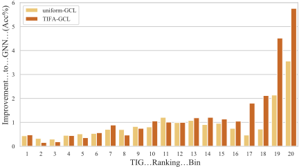
To explore why our TIFA-GCL method can benefit SSNC more than uniform-GCL, we display the comparison between TIFA-GCL with uniform-GCL at each TIG ranking bin in Figure 4. We can find that TIFA-GCL outperforms uniformGCL by a large margin at nodes with small TIG values and achieves comparable performance at nodes with large TIG values. This indicates that our TIFA-GCL can effectively strengthen the GCL's effect for nodes that are underrepresented in graph learning (small TIG value represents that node's received annotated information from topology is insufficient or confusing), thus achieving higher performance than existing uniform-GCL methods.
6 RelatedWork
The idea behind contrastive learning is to utilize selfsupervision information among contrastive pairs, which are constructed by randomly perturbation. By regularizing the perturbed representations, e.g., pulling the distance between positive pairs closer while pushing negative pairs apart, CL learns high quality representations for both images [Sohn et al., 2020] and texts [Qu et al., 2021].
In graph field, [Velickovic et al., 2019] learn node representations via mutual information maximization, which can be treated as the early applications of the idea of CL in graph. Recent GCL studies on SSNC mainly focus on three topics: (1) Devising graph-specific CL frameworks by combining GCL with different modules: such as pre-training [Qiu et al., 2020], graph generating target [Wan et al., 2021] and implicit contrastive method [Kefato and Girdzijauskas, 2021]. (2) Developing graph data augmentation methods, such as graph diffusion [Hassani and Khasahmadi, 2020], random propagation [Feng et al., 2020], subgraph aggregation [Wang and Liu, 2021], and generating from different GNN encoders [Wan et al., 2021]; and (3) Analyzing important questions in GCL, such as the augmentation method [You et al., 2020], GCL robustness [Jovanovic et al., 2021], sampling strategies [Chen et al., 2021]. However, all these existing GCL methods ignore the imbalanced annotated information distribution and apply GCL uniformly to the whole graph. Our TIFA-GCL can solve this issue by considering the TIG of different nodes.
7 Conclusion and FutureWork
In this work, we investigate contrastive learning in semisupervised node classification. We point out that current GCL methods lack consideration of the uneven distribution of annotated information, which greatly affects the graph learning performance. By analyzing the distributions of annotated information GCL contribution, we find that the benefit brought by GCL in node representation learning mainly comes from the nodes with less annotated information. Motivated by our findings, we systematically devise the TIFA-GCL framework. Extensive experiments in various scenarios demonstrate the effectiveness and generalizability of our method.
Acknowledgements
This work was supported in part by a Tencent Research Grant and National Natural Science Foundation of China (No. 62176002). Xu Sun is the corresponding author of this paper.
@inproceedings{ijcai2022p395,
  title     = {Rethinking the Promotion Brought by Contrastive Learning to Semi-Supervised Node Classification},
  author    = {Chen, Deli and Lin, Yankai and Li, Lei and Ren, Xuancheng and Li, Peng and Zhou, Jie and Sun, Xu},
  booktitle = {Proceedings of the Thirty-First International Joint Conference on
               Artificial Intelligence, {IJCAI-22}},
  publisher = {International Joint Conferences on Artificial Intelligence Organization},
  editor    = {Luc De Raedt},
  pages     = {2852--2858},
  year      = {2022},
  month     = {7},
  note      = {Main Track},
  doi       = {10.24963/ijcai.2022/395},
  url       = {https://doi.org/10.24963/ijcai.2022/395},
}
TY - CPAPER TI - Rethinking the Promotion Brought by Contrastive Learning to Semi-Supervised Node Classification AU - Chen, Deli AU - Lin, Yankai AU - Li, Lei AU - Ren, Xuancheng AU - Li, Peng AU - Zhou, Jie AU - Sun, Xu T2 - Proceedings of the Thirty-First International Joint Conference on Artificial Intelligence, IJCAI-22 PB - International Joint Conferences on Artificial Intelligence Organization PY - 2022 SP - 2852 EP - 2858 DO - 10.24963/ijcai.2022/395 UR - https://doi.org/10.24963/ijcai.2022/395 ER -Copied
Machine-readable versions of this paper, for tools and AI agents:





