
Taylor-Lagrange Neural Ordinary Differential Equations: Toward Fast Training and Evaluation of Neural ODEs
Proceedings of the Thirty-First International Joint Conference on Artificial Intelligence. Main Track. Pages 2923-2929.
https://doi.org/10.24963/ijcai.2022/405
Keywords
- Machine Learning: Recurrent Networks
- Machine Learning: Time-series; Data Streams
- Machine Learning: Other
Abstract
Neural ordinary differential equations (NODEs) -- parametrizations of differential equations using neural networks -- have shown tremendous promise in learning models of unknown continuous-time dynamical systems from data. However, every forward evaluation of a NODE requires numerical integration of the neural network used to capture the system dynamics, making their training prohibitively expensive. Existing works rely on off-the-shelf adaptive step-size numerical integration schemes, which often require an excessive number of evaluations of the underlying dynamics network to obtain sufficient accuracy for training. By contrast, we accelerate the evaluation and the training of NODEs by proposing a data-driven approach to their numerical integration. The proposed Taylor-Lagrange NODEs (TL-NODEs) use a fixed-order Taylor expansion for numerical integration, while also learning to estimate the expansion's approximation error. As a result, the proposed approach achieves the same accuracy as adaptive step-size schemes while employing only low-order Taylor expansions, thus greatly reducing the computational cost necessary to integrate the NODE. A suite of numerical experiments, including modeling dynamical systems, image classification, and density estimation, demonstrate that TL-NODEs can be trained more than an order of magnitude faster than state-of-the-art approaches, without any loss in performance.
- [Bettencourt et al., 2019] J. Bettencourt, Matthew J. John- son, and D. Duvenaud. Taylor-mode automatic differen- tiation for higher-order derivatives in jax. In Workshop on Program Transformations for ML, NeurIPS, 2019.
- [Chen et al., 2018] Ricky TQ Chen, Yulia Rubanova, Jesse Bettencourt, and David K Duvenaud. Neural ordinary dif- ferential equations. Advances in Neural Information Pro- cessing Systems, 2018.
- [Cranmer et al., 2020] M. Cranmer, Sam Greydanus, Stephan Hoyer, Peter W. Battaglia, David N. Spergel, and Shirley Ho. Lagrangian neural networks. ArXiv, abs/2003.04630, 2020.
- [Deng, 2012] Li Deng. The mnist database of handwritten digit images for machine learning research. IEEE Signal Processing Magazine, 2012.
- [Djeumou et al., 2021] Franck Djeumou, Abraham P Vinod, Eric Goubault, Sylvie Putot, and Ufuk Topcu. On-the-fly control of unknown smooth systems from limited data. In 2021 American Control Conference. IEEE, 2021.
- [Djeumou et al., 2022a] Franck Djeumou, Cyrus Neary, Eric Goubault, Sylvie Putot, and Ufuk Topcu. Neural net- works with physics-informed architectures and constraints for dynamical systems modeling. In Learning for Dynam- ics and Control. PMLR, 2022.
- [Djeumou et al., 2022b] Franck Djeumou, Cyrus Neary, Eric Goubault, Sylvie Putot, and Ufuk Topcu. Taylor-lagrange neural ordinary differential equations: Toward fast train- ing and evaluation of neural odes. ArXiv, abs/2201.05715, 2022.
- [Finlay et al., 2020] Chris Finlay, J. Jacobsen, L. Nurbekyan, and Adam M. Oberman. How to train your neural ode: the world of jacobian and kinetic regularization. In International Conference on Machine Learning. PMLR, 2020.
- [Finzi et al., 2020] Marc Finzi, Ke Alexander Wang, and Andrew G Wilson. Simplifying hamiltonian and la- grangian neural networks via explicit constraints. Ad- vances in Neural Information Processing Systems, 2020.
- [Ghosh et al., 2020] Arna Ghosh, Harkirat Singh Behl, Em- ilien Dupont, Philip H. S. Torr, and Vinay Namboodiri. Steer : Simple temporal regularization for neural odes. ArXiv, abs/2006.10711, 2020.
- [Grathwohl et al., 2019] Will Grathwohl, Ricky T. Q. Chen, Jesse Bettencourt, Ilya Sutskever, and David Kristjan- son Duvenaud. Ffjord: Free-form continuous dynam- ics for scalable reversible generative models. ArXiv, abs/1810.01367, 2019.
- [Greydanus et al., 2019] Samuel Greydanus, Misko Dzamba, and Jason Yosinski. Hamiltonian neural networks. Advances in Neural Information Processing Systems, 2019.
- [Griewank and Walther, 2008] Andreas Griewank and An- drea Walther. Evaluating derivatives: principles and tech- niques of algorithmic differentiation. SIAM, 2008.
- [Gupta et al., 2020] Jayesh K Gupta, Kunal Menda, Zachary Manchester, and Mykel Kochenderfer. Structured mechan- ical models for robot learning and control. In Learning for Dynamics and Control. PMLR, 2020.
- [Kelly et al., 2020] Jacob Kelly, Jesse Bettencourt, Matthew J Johnson, and David K Duvenaud. Learn- ing differential equations that are easy to solve. Advances in Neural Information Processing Systems, 2020.
- [Mathieu and Nickel, 2020] Emile Mathieu and Maximilian Nickel. Riemannian continuous normalizing flows. ArXiv, abs/2006.10605, 2020.
- [Menda et al., 2019] Kunal Menda, Jayesh K Gupta, Zachary Manchester, and Mykel J Kochenderfer. Struc- tured mechanical models for efficient reinforcement learning. In Workshop on Structure and Priors in Reinforcement Learning, International Conference on Learning Representations, 2019.
- [Pal et al., 2021] Avik Pal, Yingbo Ma, Viral Shah, and Christopher V Rackauckas. Opening the blackbox: Ac- celerating neural differential equations by regularizing in- ternal solver heuristics. In International Conference on Machine Learning. PMLR, 2021.
- [Papamakarios et al., 2017] George Papamakarios, Iain Murray, and Theo Pavlakou. Masked autoregressive flow for density estimation. ArXiv, abs/1705.07057, 2017.
- [Poli et al., 2020] Michael Poli, Stefano Massaroli, Atsushi Yamashita, Hajime Asama, and Jinkyoo Park. Hyper- solvers: Toward fast continuous-depth models. ArXiv, abs/2007.09601, 2020.
- [Roe et al., 2005] Byron P Roe, Hai-Jun Yang, Ji Zhu, Yong Liu, Ion Stancu, and Gordon McGregor. Boosted decision trees as an alternative to artificial neural networks for par- ticle identification. Nuclear Instruments and Methods in Physics Research Section A: Accelerators, Spectrometers, Detectors and Associated Equipment, 2005.
- [Salman et al., 2018] Hadi Salman, Payman Yadollahpour, Tom Fletcher, and Nematollah Batmanghelich. Deep dif- feomorphic normalizing flows. ArXiv, abs/1810.03256, 2018.
- [Zhong et al., 2021] Yaofeng Desmond Zhong, Biswadip Dey, and Amit Chakraborty. Benchmarking energy- conserving neural networks for learning dynamics from data. In Learning for Dynamics and Control. PMLR, 2021.
References were extracted automatically from the PDF and may contain errors.
Full text extracted automatically from the PDF; figures, tables and equations may differ. The PDF is the version of record.
1 Introduction
Neural ordinary differential equations (NODEs) have recently shown tremendous promise as a means to learn unknown continuous-time dynamical systems from trajectory data [Chen et al., 2018]. By parametrizing differential equations as neural networks, as opposed to directly fitting the available trajectory data, NODEs provide compact representations of continuous-time systems that are memory-efficient and that are well understood; they allow the user to harness an existing wealth of knowledge from applied mathematics, physics, and engineering. For example, recent works have used NODEs as a means to incorporate physics-based knowledge into the learning of dynamical systems [Djeumou et al., 2022a; Menda et al., 2019; Gupta et al., 2020; Cranmer et al., 2020; Greydanus et al., 2019; Finzi et al., 2020; Zhong et al., 2021]. Furthermore, NODEs have been used to define continuous normalizing flows - a class of invertible density models - to learn complex probability distributions over data [Chen et al., 2018; Grathwohl et al., 2019; Mathieu and Nickel, 2020; Salman et al., 2018].
∗These authors contributed equally.
The code is available at https://github.com/wuwushrek/TayLaNets.
However, the training of NODEs can become prohibitively expensive [Grathwohl et al., 2019; Kelly et al., 2020; Finlay et al., 2020]. In particular, every forward evaluation of the NODE requires the numerical integration of the underlying neural network parametrizing the system dynamics. Existing methods for the training of NODEs use off-the-shelf adaptive step-size numerical integration schemes for this purpose. However, in order to obtain sufficient accuracy, such integration schemes have been shown in practice to require an excessive number of evaluations of the underlying neural network. Furthermore, the severity of this problem has been shown to grow as the training of the neural ODE progresses; while the neural ODE learns to fit the available data, it does not learn a representation of the dynamics that is easy to integrate [Finlay et al., 2020]. These computational issues render the training of neural ODEs on large datasets intractable, and they also prevent neural ODEs from being deployed in applications requiring repeated fast online predictions; such as for model-predictive control of robotic systems.

To address the above issues, we present Taylor-Lagrange NODEs (TL-NODEs); we use a truncated Taylor expansion of the underlying neural network to predict the future system state, and we train a separate neural network to correct this prediction according to the Lagrange form of the expansion's remainder. By training the second corrector network, the approach significantly reduces the computational cost necessary for accurate numerical integration, while ensuring little-tono-loss in the accuracy of the model. Figure 2 illustrates the major components of TL-NODE, which are discussed below.
(1) Taylor expansions for the numerical integration of the NODE. In order to integrate the NODE, we use a fixedorder Taylor expansion of the dynamical system in time. We take advantage of Taylor-mode automatic differentiation to efficiently compute the higher-order terms of the expansion on a GPU [Bettencourt et al., 2019]. By specifying the number of terms to include in the expansion, we ensure that only a fixed number of evaluations of the underlying dynamics network are required per training step.
(2) Correcting the expansion's approximation error. We use the Lagrange form of the expansion's remainder to define a correction term, which greatly improves the accuracy of the predictions obtained from the truncated expansion. To estimate this approximation error efficiently, we propose to use a neural network to predict the so-called midpoint value - a point near the center of the expansion at which the approximation error can be evaluated exactly. While learning this midpoint value may, in general, be as complex as learning the neural ODE itself, we derive explicit formulas for the midpoint using assumptions on the regularity of the dynamics. These expressions reduce the complexity of the learning problem; only one unknown term in the expression must be learned. We provide upper bounds on the error of the proposed Taylor-Lagrange expansion, in terms of the error in the predicted midpoint value and the order of the expansion.
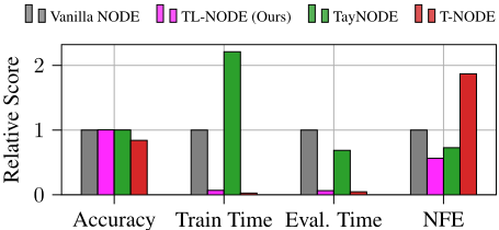
We demonstrate the effectiveness of the proposed approach through a suite of numerical experiments. The experimental tasks include the integration of known dynamics, learning to predict unknown dynamics, supervised classification, and density estimation. Figure 1 illustrates the result of applying TL-NODE to a classification task. Across all experiments we observe that the training and the evaluation of TL-NODEs is more than an order of magnitude faster than existing NODE methods, while incurring no loss in performance.
Related Work. Similarly to our work, a number of papers study how to reduce the computational cost of training neural ODEs. After [Chen et al., 2018] initially presented the neural ODE, [Grathwohl et al., 2019] proposed a stochastic estimator of the likelihood to reduce computational cost when using neural ODEs for continuous normalizing flows. [Kelly et al., 2020; Finlay et al., 2020; Pal et al., 2021] propose additional regularization terms to learn neural ODEs that are easy to integrate. [Ghosh et al., 2020] propose to regularize the neural ODE by randomly sampling the end time of the ODE during training. However, all of these works use off-the-shelf numerical integration algorithms for the forward evaluation of the NODE. By contrast, our work suggests a novel data-driven integration scheme, resulting in training times that are an order of magnitude faster than the current state-of-the-art.
Meanwhile, [Poli et al., 2020] also suggest training an additional corrector neural network to speed up the numerical integration of NODEs. However, they do not present a technique that is able to apply such a corrector network during the training of the NODE. By contrast, we propose algorithms for the simultaneous training of the dynamics network and the remainder estimation network; this simultaneous training results not only in a speedup of the NODE evaluations, but also in a speedup of the NODE's training. Furthermore, we propose a method to simplify the learning of the remainder term by taking advantage of regularity assumptions on the system dynamics. This simplification leads to more efficient and generalizable learning of the correction term.
2 Background
We begin by introducing necessary background on ordinary differential equations (ODEs) and on neural ODEs.
Ordinary Differential Equations (ODEs). Let the function f(x, t) : Rn ×R+ ↦→ Rn be Lipschitz-continuous in x and t. An ordinary differential equation specifies the instantaneous change of a vector-valued signal of time x : R+ ↦→ Rn .
We note that in general, the explicit dependence of f(x, t) on t can be removed by adding a dimension to the state variable x. As such, throughout the remainder of the paper, we consider autonomous systems of the form ˙x(t) = f(x(t)). Furthermore, for notational simplicity we use the subscript notation xt in place of x(t).
Given some initial state x0 := xt0 ∈ Rn at initial time t0 ≥ 0, we wish to compute a solution to (1). In this work, we are specifically interested in predicting the value of the state xt, at an arbitrary future point in time T ≥ t0. The value of xT can be found by integrating or solving the ODE: xT = x0 + ∫ T t0 f(xs) ds.
Neural Ordinary Differential Equations (NODEs). Neural ODEs (NODEs) are a class of deep learning models that use a neural network fθ(x) to parametrize an ODE, and that subsequently use numerical integration algorithms to evaluate the model's outputs. More specifically, given a NODE input tuple (x0, t0, T) consisting of an initial state x0, an initial time t0, and a prediction time T, the output ˆxT := NODEθ(x0, t0, T) of the NODE with parameter vector θ is given by ODESolve(fθ, x0, t0, T) ≈ x0 + ∫ T t0 fθ(xs)ds. Here, ODESolve(fθ, x0, t0, T ) is a numerical approximation of the solution to the dynamics parametrized by fθ(x).
We note that the particular algorithm used in place of ODESolve(·) influences the model's accuracy, the computational cost of forward evaluations of the model, and the computational cost of training the model. Existing implementations of neural ODEs have typically relied on existing adaptive-step numerical integration algorithms for this purpose. By contrast, this work proposes the use of a novel Taylor expansion based method that uses data-drive estimations of the expansion's truncation error to evaluate and train neural ODEs efficiently and accurately.
3 Taylor-Lagrange Neural Ordinary Differential Equations (TL-NODE)
In this section we propose TL-NODEs for the efficient and accurate training and evaluation of neural ODEs.
3.1 Data-Driven Taylor-Lagrange Numerical Integration of the NODE Dynamics
Our objective is to efficiently and accurately evaluate neural ODEs through numerical integration of fθ(·). Toward this end, we propose to make direct use of the Taylor-Lagrange expansion of xt in time. Taylor expansions are techniques used to approximate a function near a particular expansion point using polynomials. We use the term Taylor-Lagrange expansion to refer to the truncated Taylor expansion including the Lagrange form of the remainder. In order to obtain highly accurate expansions of xt without requiring an excessive number of evaluations of fθ(·), we propose to train a separate neural network with parameters ϕ to estimate the remainder term in the expansion. We give a step-by-step description of the proposed methodology below.
Partitioning the prediction interval. We begin by partitioning the prediction interval [t0, T] into a collection of H sub-intervals [ti, ti+1]. For notational convenience, we assume the value of the integration time step is fixed, i.e. ∆t = ti+1 - ti for all i = 0, . . . ,H - 1. Given the value of the state xti at time ti, we compute an approximation of the value of the state at the next time step ˆxti+1 via a pth order Taylor-Lagrange expansion of xt about time ti, which we denote by TL∆t θ,ϕ (xti ). The output TLNODEθ,ϕ(x0, t0, T) of the neural ODE is computed by iteratively using TL∆t θ,ϕ (·) to approximate the integral of fθ(·) over each sub-interval.
Expressing TL∆t θ,ϕ(·) in Terms of fθ(·). Note that because fθ(x) estimates the time derivative of the system state x, the Taylor-Lagrange expansion of xt may be expressed in terms of the Taylor coefficients f [l] θ (x), which are recursively defined through the equations f [1] θ (x) = fθ(x) and f [l+1] θ (x) = 1 l+1 [ ∂f [l] θ ∂x fθ](x). Equation (2) accordingly presents the Taylor-Lagrange expansion of xt about the point in time ti, evaluated at the future time ti+1 = ti +∆t.
The first two terms on the right hand side of (2) make up the truncated Taylor expansion of xt, while Rϕ(fθ, xti , ∆t) denotes an estimation of the remainder of this truncated expansion. More specifically, Rϕ(fθ, xti , ∆t) estimates the approximation error of the pth order expansion; if we could known this value exactly, (2) would provide an exact evaluation of the integral xti + ∫ ti+1 ti fθ(xs)ds. Belowwe propose a methodology to learn to accurately estimate the value of this remainder term, given fθ, xti , and ∆t as inputs.
Estimating the Remainder Term Rϕ(·). To obtain accurate and generalizable estimations of the remainder term Rϕ(fθ, xti ,∆t), we begin by using Taylor's theorem to express it as Rϕ(fθ, xti , ∆t) = f [p] θ (Γ). Here, Γ ∈ Rn denotes the midpoint of the Taylor-Lagrange expansion. More specifically, there exists some point in time ξ with ti ≤ ξ ≤ ti+1 such that when we define Γ := xξ, then ∆tp f [p] θ (Γ) provides the exact value of the approximation error of the expansion.
While no closed form expression for the midpoint Γ exists, we propose to learn to predict its value given the state xti and the time step ∆t. Learning to predict Γ directly as a function of these inputs is a challenging problem in general. We instead propose to use the result of Theorem 1, which provides a closed-form expression for Γ in terms of some unknown term ¯Γ ∈ Rn . By taking advantage of this expression for Γ, we greatly simplify the task of learning to predict its value.
Theorem 1 (Simplified Midpoint Expression). If fθ is a Lipschitz-continuous function, then there exists a function ¯Γ : Rn × R+ → Rn×n such that the midpoint value Γ of the Taylor-Lagrange expansion TL∆t θ,ϕ (xti ) is related to xti , fθ(xti ), and ¯Γ(xti ,∆t) through
where ⊙ denotes matrix-vector multiplication.
Algorithm 1 Evaluating TLNODEθ,ϕ(x0, t0, T )
Input: x0, t0, T
Parameter: θ, ϕ, p, H
Output: Model prediction ˆxT .
- 1: ˆxt0 ← x0; ∆t ← T-t0 H
- 2: for i = 0, 1, . . . ,H do{ ti ← t0 + i∆t}
- 3: for i = 0, 1, . . . ,H -1 do
- 4: Γ← ˆxti + ¯Γϕ(ˆxti ,∆t) ⊙ fθ(ˆxi)
- 5: ˆxti+1 ← ˆxti + ∑p-1 l=1 ∆tl f [l] θ (ˆxi) +∆tp f [p] θ (Γ)
- 6: end for
- 7: return ˆxH
Theorem 1 is obtained using tools from interval TaylorLangrange based reachability analysis [Djeumou et al., 2021]. More specifically, the equation given in (3) is derived from explicit formulas for the so-called apriori enclosure - a set derived from the local Lipschitzness of fθ that is guaranteed to contain the value of TL∆t θ,ϕ (xti ). A proof of Theorem 1 is provided in the extended version of the paper [Djeumou et al., 2022b]. We also prove that for linear dynamics, ¯Γ does not depend on xti .
Estimating the Midpoint Value. Given the result of Theorem 1, we propose to parameterize the unknown function ¯Γϕ(·) using a neural network with parameters ϕ. For notational simplicity, we use Γϕ(x,∆t) to denote the value of the right hand side of (3) when ¯Γ(·) is approximated by ¯Γϕ(·). Given the predicted midpoint value Γϕ(x,∆t), we estimate the remainder term of the pth order Taylor-Lagrange expansion T L∆t θ,ϕ (xti ) as Rϕ(fθ , xti , ∆t) ≈ ∆tp f [p] θ (Γϕ(xti ,∆t)).
The Proposed TL-NODE Evaluation Algorithm. Algorithm 1 summarizes the proposed approach for the numerical evaluation of neural ODEs. In lines 1 and 2, the prediction interval [t0, T] is broken into H sub-intervals. The for loop in lines 3 - 6 iterates over these sub-intervals, and uses the midpoint prediction network Γϕ(·) to estimate the midpoint value (line 4), before using this estimate to approximate the state value ˆxti+1 at the end of the sub-interval (line 5).
Bounding the Error of the TL-NODE Evaluation Algorithm. Given a fixed dynamics function fθ(·), we seek to bound the error on a pth order Taylor-Lagrange expansion which uses a learned midpoint value predictor Γϕ(·) to estimate the expansion's remainder Rϕ(·). Such an error bounds straightforwardly depends on how well Γϕ(·) approximates the true midpoint Γ, as described in Theorem 2. A proof of Theorem 2 is provided in the Appendix.
Theorem 2 (Integration Accuracy). If the learned midpoint predictor Γϕ(·) is a O(η) approximator to the midpoint Γ of the Taylor-Lagrange expansion of TL∆t θ,ϕ (xti ), then ∥xti+1 - T L∆t θ,ϕ (xti )∥ ≤ cη∆tp for some c > 0 that depends on fθ.
A Note on the Evaluating the Taylor Coefficients. The Taylor coefficients f [1] θ (·), . . . , f [p] θ (·) can in principle be evaluated using repeated application of forward-mode automatic differentiation to iteratively compute the Jacobianvector products [ ∂f [l] θ ∂x fθ](x). However, doing so would incur a time cost of O(exp(p)). We instead use Taylor mode automatic differentiation, which computes the first p Taylor coefficients f [1] θ (·), . . . , f [p] θ (·) in a single pass, with a time cost of only O(p2 ) or of O(p log p), depending on the underlying operations involved [Griewank and Walther, 2008; Bettencourt et al., 2019; Kelly et al., 2020].
3.2 Training Taylor-Lagrange Neural Ordinary Differential Equations
Given a training dataset D, we wish to train both components of the TL-NODE: the dynamics network fθ(·) and the midpoint prediction network Γϕ(·). To do so, we propose an algorithm that alternates between training each of the components via stochastic gradient descent while keeping the parameters of the other component fixed. We assume that each datapoint within the dataset D = {(xj0 , tj0 , T j , yj )}|D| j=1 is comprised of an initial state xj , an initial time tj0 , a prediction time T j , and a labeled output value yj .
Training the Dynamics Network fθ(·). We begin by holding the parameter vector ϕ of the midpoint prediction network to some fixed value ˆ ϕ, and training the dynamics network fθ(·) by solving the optimization problem (4) via stochastic gradient descent.
Here, L(·) is any differentiable loss function and ˆxti denotes integrator-estimated intermediate state at time ti.
The summation in the second line of (4) measures the magnitude of the remainder terms Rϕ(·) of the truncated TaylorLagrange expansions used for numerical integration. We may interpret this penalty term as having two purposes. Firstly, it acts as a regularizer that penalizes the higher-order derivatives of fθ(·) during training. Intuitively, by penalizing these higher order derivatives we encourage solutions that fit the data while also remaining as simple as possible. Secondly, the penalty term prevents the TL-NODE from using Rϕ(·) to overfit the training data. By ensuring that the remainder term of the Taylor-Lagrange expansion remains small during training, we learn a dynamics function fθ(·) whose truncated expansions fit the training data as well as possible, while using Rϕ(·) only for small corrections.
Training the Midpoint Prediction Network Γϕ(·). Recall that the midpoint prediction network Γϕ(·) plays a crucial role in accurately integrating the dynamics specified by fθ(·). So, as the parameters of the dynamics network fθ(·) are updated throughout training, our estimates of Γ, the midpoint of the Taylor-Lagrange expansion of fθ(·), should be updated accordingly. We thus propose to occasionally freeze the parameters of the dynamics network ˆ θ in order to train Γϕ(·).
After fixing ˆ θ, we begin by generating a small dataset Dˆ θ . The datapoints of Dˆ θ correspond to solutions of the
Algorithm 2 Training the TL-NODE
Input: Training dataset D
Parameter: Nθ, Nϕ, Ntrain, N|Dˆ θ |
Output: Model parameters θ, ϕ
- 1: Initialize parameters θ, ϕ
- 2: for Ntrain steps do
- 3: Fix ˆ ϕ ← ϕ
- 4: for Nθ steps do{ θ ← sgdStep(Eq. (4), θ, ˆ ϕ, D)}
- 5: Fix ˆ θ ← θ; {(xj0 , tj0 , T j )}j ← Sample(D, N|Dˆ θ |)
- 6: Dˆ θ ← ODESolve(fˆ θ , {(xj0 , tj0 , T j )}j )
- 7: for Nϕ steps do{ ϕ ← sgdStep(Eq. (5), ˆ θ, ϕ, Dˆ θ )}
- 8: end for
- 9: return θ, ϕ
ODE encoded by the fixed dynamics network fˆ θ (·). That is, for each (x0, t0, T, y) ∈ Dˆ θ the output label y is given by ODESolve(fˆ θ , x0, t0, T ), where ODESolve(·) is a highly accurate adaptive-step ODE solver. Once the dataset Dˆ θ has been generated, we train Γϕ(·) by using stochastic gradient descent to solve the optimization problem (5).
The Proposed TL-NODE Training Algorithm. Algorithm 2 details the proposed training procedure. Throughout training we alternate between the following two subroutines: (lines 3-4) fix ϕ and take Nθ stochastic gradient descent steps to train the dynamics network fθ(·) according to (4), (lines 57) fix θ and take Nϕ stochastic gradient descent steps to train the midpoint prediction network Γϕ(·) according to (5).
4 Numerical Experiments
We demonstrate the effectiveness of TL-NODE through several numerical experiments: the numerical integration of known dynamics, the learning of unknown dynamics, a supervised classification task, and a density estimation task. As an initial illustrative example we apply TL-NODE to linear dynamics. However, we note that the latter classification and density estimation tasks involve non-linear, time-dependent, and high-dimensional dynamics. Additional experimental details - including hyperparameter selection - are included in the extended version of the paper [Djeumou et al., 2022b].
4.1 Modeling a Dynamical System
We begin by applying TL-NODE to the task of modeling a stiff dynamical system. More specifically, we use the proposed Taylor-Lagrange approach to learn, and to integrate, the ODE ˙x = Ax, where x ∈ R2 and A ∈ R2×2 has eigenvalues λ1 = -1 and λ2 = -1000.
Integration of Known Stiff Dynamics.
To examine the accuracy and robustness of the midpoint prediction network Γϕ(·), we begin by assuming the dynamics function f(x) = Ax is known, and we use the proposed Taylor-Lagrange numerical integration method to predict future system states. We note that because we assume f(·) is known, there is no need to parameterize the system dynamics using a neural network fθ(·). However, we may still apply the method outlined in §3.2 to train Γϕ(·) to predict the approximation error of the Taylor-Lagrange expansions.
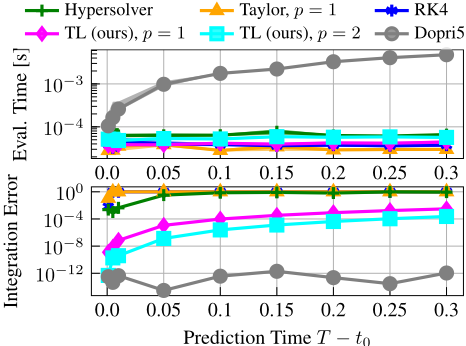
Baselines. We apply both 1st and 2nd order Taylor expansions for numerical integration. For comparison, we include the results of a fixed-step RK4 method, an adaptivestep method (Dopri5), and the Hypersolver method [Poli et al., 2020]. The tolerance parameters rtol and atol of the adaptive-step Dopri5 integrator are both set to 1.4e-12 . We also plot the result of using a Taylor expansion for integration, without including the learned approximation error term.
Results. Figure 3 illustrates the numerical integration results. For brevity, in the figure we refer to the proposed Taylor-Lagrange method for integration as TL. We observe that TL-NODE enjoys lower integration error than all of the baseline methods except for Dopri5. However, Dopri5 requires computation times that are more than an order of magnitude higher than that of our method. We additionally observe that while the Hypsersolver method requires similar computation time to TL-NODE, the error of its numerical integration results are several orders of magnitude higher. Furthermore, we note that for any prediction time intervals T - t0 larger than 0.05(s), the fixed-step RK4, Truncated Taylor expansion method, and Hypersolver method all have normalized prediction errors values of 1.0 (the highest possible value). By contrast, our TL-NODE approach achieves an average error value on the order of 10-4 , even when T - t0 = 0.3(s). This demonstrataes the robustness of the proposed approach to the size of the prediction interval.
Finally, we note that the integration error of the truncated Taylor expansion method (yellow) is several orders of magnitude larger than that of TLN. The only difference between these methods is TLN's inclusion of the proposed correction term that learns the approximation error, demonstrating the gain in accuracy that this learned correction term provides.
| Method | Train Accuracy (%) | Test Accuracy (%) | Train Time (min) | Eval. Time (ms) | NFE |
|---|---|---|---|---|---|
| TL-NODE (ours) | 99.96 | 98.23 | 2.55 | 1.04 | 62 |
| Vanilla NODE | 99.33 | 97.87 | 42.7 | 16 | 110.6 |
| TayNODE | 99.29 | 98.02 | 94.3 | 11 | 80.00 |
| RNODE | 98.72 | 97.74 | 10.2 | 2.05 | 98.0 |
| SRNODE* | 100.0 | 98.08 | 98.1 | - | 259.0 |
| STEER* | 100.0 | 97.94 | 103 | - | 265.0 |
Learning Unknown Dynamics
We now assume that the system dynamics f (x) = Ax are unknown and train a TL-NODE to model the dynamical system.
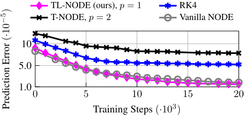
Baselines. We compare to Vanilla NODE, which uses adaptive-step Dopri5 for numerical integration, to a NODE trained using fixed-step RK4, and to T-NODE - a version of our approach that also uses Taylor expansions for integration, but does not estimate their remainder term.
Results. Figure 4 illustrates the NODE's average prediction error as a function of the number of elapsed training steps. TL-NODE achieves smiliar prediction error values to the Vanilla NODE throughout training, while the prediction errors of the other two baseline methods are twice as large. The wall-clock training time for TL-NODE is 31.9s, for the Vanilla NODE it is 609.8s, for the RK4 NODE it is 35.8s, and for T-NODE it is 21.2s. Algorithm 2 effectively balances the training of TL-NODE's two components: fθ(·) and Γϕ(·). The result is a dynamics model that is as accurate as the Vanilla NODE trained using Dopri5, but whose training and evaluation times are much faster.
4.2 Supervised Classification
We train a TL-NODE model to perform classification on the MNIST dataset [Deng, 2012]. Our model follows the architecture of the neural ODE-based MNIST classifier presented in the work of [Kelly et al., 2020] and further used in [Pal et al., 2021] for benchmarking. Specifically, the model uses a two-layered neural network of size 100 and 728 (size of the images) with sigmoid-based non linearities to parameterize the dynamics function fθ(·). The NODE outputs propagate through a linear classifier to estimate of the image labels.
Baselines. We compare the proposed Taylor-Lagrange networks with state-of-the-art NODE algorithms. More specifically, we compare to RNODE [Finlay et al., 2020] and TayNode [Kelly et al., 2020] using the source code provided by the respective authors. We implicitly also compare our results with other regularization techniques such STEER [Ghosh et al., 2020] and SRNODE [Pal et al., 2021] thanks to the thorough experiments provided in [Pal et al., 2021] for a similar model of the MNIST classification problem.
Results. Table 1 lists the experimental results. TL-NODE achieves evaluation and training times that are more than an order of magnitude faster than the baseline approaches, while also achieving the highest accuracy on the test dataset. TLNODE also learns a dynamics network fθ(·) that requires the smallest number of function evaluations (NFE) when it is being numerically integrated using an adaptive-step integrator. The low NFE score of TL-NODE indicates that the regularization term in (4) is effective at producing learned dynamics networks fθ(·) that are easy to numerically integrate.
4.3 Density Estimation
We apply TL-NODEs to train continuous-normalizing-flowbased generative models [Chen et al., 2018; Grathwohl et al., 2019] to approximate the distribution of the MiniBooNE dataset [Roe et al., 2005; Papamakarios et al., 2017].
| Method | Loss (nat) | Train Time (min) | NFE |
|---|---|---|---|
| TL-NODE (ours) | 9.62 | 12.3 | 167.9 |
| Vanilla NODE | 9.74 | 59.7 | 183.8 |
| TayNODE | 9.75 | 148.3 | 168.2 |
| RNODE | 9.78 | 10.32 | 182.0 |
Results. TL-NODE achieves the best loss score and the lowest required number of function evaluations (NFE) in comparison with the baseline approaches.
5 Conclusions
We present Taylor-Lagrange Neural Ordinary Differential Equations (TL-NODEs): a class of neural ODEs (NODEs) that use fixed-order Taylor expansions for numerical integration during NODE training and evaluation. TL-NODEs also train a separate neural network to predict the expansion's remainder, which is used as a correction term to improve the accuracy of the NODE's outputs. We demonstrate that TLNODEs enjoy evaluation and training times that are an order of magnitude faster than the current state-of-the-art, without any loss in accuracy. Future work will aim to apply the accelerated NODE evaluation times to the online model-based control of unknown dynamical systems.
Acknowledgements
This work was supported in part by ARL W911NF2020132, AFOSR FA9550-19-1-0005, and NSF 1646522.
@inproceedings{ijcai2022p405,
  title     = {Taylor-Lagrange Neural Ordinary Differential Equations: Toward Fast Training and Evaluation of Neural ODEs},
  author    = {Djeumou, Franck and Neary, Cyrus and Goubault, Eric and Putot, Sylvie and Topcu, Ufuk},
  booktitle = {Proceedings of the Thirty-First International Joint Conference on
               Artificial Intelligence, {IJCAI-22}},
  publisher = {International Joint Conferences on Artificial Intelligence Organization},
  editor    = {Luc De Raedt},
  pages     = {2923--2929},
  year      = {2022},
  month     = {7},
  note      = {Main Track},
  doi       = {10.24963/ijcai.2022/405},
  url       = {https://doi.org/10.24963/ijcai.2022/405},
}
TY - CPAPER TI - Taylor-Lagrange Neural Ordinary Differential Equations: Toward Fast Training and Evaluation of Neural ODEs AU - Djeumou, Franck AU - Neary, Cyrus AU - Goubault, Eric AU - Putot, Sylvie AU - Topcu, Ufuk T2 - Proceedings of the Thirty-First International Joint Conference on Artificial Intelligence, IJCAI-22 PB - International Joint Conferences on Artificial Intelligence Organization PY - 2022 SP - 2923 EP - 2929 DO - 10.24963/ijcai.2022/405 UR - https://doi.org/10.24963/ijcai.2022/405 ER -Copied
Machine-readable versions of this paper, for tools and AI agents:





