
Non-Cheating Teaching Revisited: A New Probabilistic Machine Teaching Model
Proceedings of the Thirty-First International Joint Conference on Artificial Intelligence. Main Track. Pages 2973-2979.
https://doi.org/10.24963/ijcai.2022/412
Keywords
- Machine Learning: Learning Theory
- Machine Learning: Probabilistic Machine Learning
Abstract
Over the past decades in the field of machine teaching, several restrictions have been introduced to avoid ‘cheating’, such as collusion-free or non-clashing teaching. However, these restrictions forbid several teaching situations that we intuitively consider natural and fair, especially those ‘changes of mind’ of the learner as more evidence is given, affecting the likelihood of concepts and ultimately their posteriors. Under a new generalised probabilistic teaching, not only do these non-cheating constraints look too narrow but we also show that the most relevant machine teaching models are particular cases of this framework: the consistency graph between concepts and elements simply becomes a joint probability distribution. We show a simple procedure that builds the witness joint distribution from the ground joint distribution. We prove a chain of relations, also with a theoretical lower bound, on the teaching dimension of the old and new models. Overall, this new setting is more general than the traditional machine teaching models, yet at the same time more intuitively capturing a less abrupt notion of non-cheating teaching.
- [Balbach, 2008] Frank J Balbach. Measuring teachability us- ing variants of the teaching dimension. Theoretical Com- puter Science, 397(1-3):94-113, 2008.
- [Doliwa et al., 2010] Thorsten Doliwa, Hans Ulrich Simon, and Sandra Zilles. Recursive teaching dimension, learning complexity, and maximum classes. In International Con- ference on Algorithmic Learning Theory, pages 209-223. Springer, 2010.
- [Doliwa et al., 2014] Thorsten Doliwa, Gaojian Fan, Hans Ulrich Simon, and Sandra Zilles. Recursive teaching dimension, VC-dimension and sample compression. The Journal of Machine Learning Research, 15(1):3107-3131, 2014.
- [Eaves-Jr. and Shafto, 2016] Baxter S Eaves-Jr. and Patrick Shafto. Toward a general, scaleable framework for bayesian teaching with applications to topic models. CoRR, 2016.
- [Gao et al., 2017a] Ziyuan Gao, David Kirkpatrick, Christoph Ries, Hans Simon, and Sandra Zilles. Preference-based teaching of unions of geometric objects. In Proceedings of the 28th International Conference on Algorithmic Learning Theory, volume 76 of Proceedings of Machine Learning Research, pages 185-207. PMLR, 15-17 Oct 2017.
- [Gao et al., 2017b] Ziyuan Gao, Christoph Ries, Hans Ul- rich Simon, and Sandra Zilles. Preference-based teaching. Journal of Machine Learning Research, 18:31:1-31:32, 2017.
- [Goldman and Kearns, 1995] Sally A Goldman and Michael J Kearns. On the complexity of teaching. Journal of Computer and System Sciences, 50(1):20-31, 1995.
- [Goldman and Mathias, 1996] Sally A Goldman and H David Mathias. Teaching a smarter learner. Journal of Computer and System Sciences, 52(2):255-267, 1996.
- [Hernández-Orallo and Telle, 2020] Jose Hernández-Orallo and Jan Arne Telle. Finite and confident teaching in ex- pectation: Sampling from infinite concept classes. In ECAI 2020, pages 1182-1189. IOS Press, 2020.
- [Khan et al., 2011] Faisal Khan, Xiaojin Zhu, and Bilge Mutlu. How do humans teach: on curriculum learning and teaching dimension. In Proceedings of the 24th In- ternational Conference on Neural Information Processing Systems, pages 1449-1457, 2011.
- [Kirkpatrick et al., 2019] David Kirkpatrick, Hans U Simon, and Sandra Zilles. Optimal collusion-free teaching. In Al- gorithmic Learning Theory, pages 506-528. PMLR, 2019.
- [Liu et al., 2017] Weiyang Liu, Bo Dai, Ahmad Humayun, Charlene Tay, Chen Yu, Linda B. Smith, James M. Rehg, and Le Song. Iterative machine teaching. In Proceedings of the 34th International Conference on Machine Learn- ing, pages 2149-2158. PMLR, 2017.
- [Mansouri et al., 2019] Farnam Mansouri, Yuxin Chen, Ara Vartanian, Jerry Zhu, and Adish Singla. Preference-based batch and sequential teaching: Towards a unified view of models. Advances in Neural Information Processing Sys- tems, 32:9199-9209, 2019.
- [Moran et al., 2015] Shay Moran, Amir Shpilka, Avi Wigderson, and Amir Yehudayoff. Compressing and teaching for low VC-dimension. In Symposium on Foundations of Computer Science, pages 40-51, 2015.
- [Shafto et al., 2014] Patrick Shafto, Noah D. Goodman, and Thomas L. Griffiths. A rational account of pedagogi- cal reasoning: Teaching by, and learning from, examples. Cognitive Psychology, 71:55 -89, 2014.
- [Wallace and Dowe, 1999] C. S. Wallace and D. L. Dowe. Minimum message length and Kolmogorov complexity. Computer Journal, 42(4):270-283, 1999.
- [Yang and Shafto, 2017] Scott Cheng-Hsin Yang and Patrick Shafto. Explainable artificial intelligence via bayesian teaching. In NIPS 2017 workshop on Teaching Machines, Robots, and Humans, pages 127-137, 2017.
- [Yang et al., 2021] Scott Cheng-Hsin Yang, Wai Keen Vong, Ravi B Sojitra, Tomas Folke, and Patrick Shafto. Mit- igating belief projection in explainable artificial intelli- gence via bayesian teaching. Scientific reports, 11(1):1- 17, 2021.
- [Zhu et al., 2018] Xiaojin Zhu, Adish Singla, Sandra Zilles, and Anna N Rafferty. An overview of machine teaching. arXiv preprint arXiv:1801.05927, 2018.
- [Zhu, 2013] Xiaojin Zhu. Machine teaching for bayesian learners in the exponential family. In Neural Information Processing Systems 26, pages 1905-1913.
- Curran, 2013.
- [Zilles et al., 2011] Sandra Zilles, Steffen Lange, Robert Holte, and Martin Zinkevich. Models of cooperative teach- ing and learning. Journal of Machine Learning Research, 12(Feb):349-384, 2011.
References were extracted automatically from the PDF and may contain errors.
Full text extracted automatically from the PDF; figures, tables and equations may differ. The PDF is the version of record.
1 Introduction
In machine teaching [Zhu et al., 2018], what we may also call algorithmic teaching, the goal of the teacher is to find an optimal witness, a collection of labelled examples, that will steer the learner toward a target concept. An important complexity notion is the teaching dimension (TD) of a concept class C, which is the minimum number of examples, from a set of ground elements X, needed to teach any concept in the class. As the teaching complexity depends on the protocol between teacher and learner and their shared information, different teaching models lead to different values for the teaching dimension.
Over the last quarter century several teaching models have been proposed, for example, the classical teaching (CT) model [Goldman and Kearns, 1995], the optimal teacher (OT) model [Balbach, 2008], recursive teaching (RT) [Zilles et al.,
∗Contact Author
2011; Doliwa et al., 2010; Doliwa et al., 2014], preferencebased teaching (PBT) [Gao et al., 2017b; Gao et al., 2017a], and non-clashing teaching (NCT) [Kirkpatrick et al., 2019]. In all these models, the teacher T : C → W is viewed as a mapping from concepts c ∈ C to witness w ∈ W (usually sets of possibly labelled examples from X) and the learner L : W → C as a partial mapping in the opposite direction. Moreover, the examples T(c) employed to teach concept c must be consistent with c, and the guessed concept L(w) when given example set w must also be consistent with w. A successful teacher-learner pair has L(T (c)) = c for any concept in the class.
Clearly, any formal model of teaching must disallow cheating, or unfair collusion between teacher and learner. As described by Moran et al [Moran et al., 2015], "roughly speaking, a collusion occurs when teacher and student agree in advance on some unnatural encoding of information about the concept c using the bit description of the chosen examples, instead of using attributes that separate c from the other concepts". Goldman and Mathias [1996] proposed that a model should be called collusion-free if whenever T(c) ⊆ w and w is consistent with c, denoted by c |= w, then also L(w) = L(T(c)) = c (hereafter called GM-collusion-free). Many abstract teaching models in the literature were introduced specifically to improve the teaching complexity of previous models while remaining GM-collusion-free. For example, the five models mentioned above (CT, OT, RT, PBT and NCT), in this order, have strictly improving teaching complexities, and all remain GM-collusion-free. The nonclashing model is provably the end of this line, as it can be shown that if every concept in class C can be taught with at most k examples by some GM-collusion-free model then the same holds for the non-clashing model, since the nonclashing model actually adheres to no other constraints than those formulated by the Goldman and Mathias condition.
Note that in a GM-collusion-free model a learner guessing c is not allowed to change its mind if given additional examples consistent with c. Consider a learner that sees the witness w = {3}, composed of one single ground element 3 ∈ X = N, and assigns some plausibility to the hypothesis that the underlying concept is the set of odd numbers codd. Some other plausibility is given to other hypotheses, such as the powers of three cpow3, the prime numbers cprime, etc. Based on simplicity of consistent concepts, the learner guesses codd. Now, if the same learner sees the witness {3, 29} or {3, 11}, the powers of three is ruled out. But the likelihood of these examples for cprime now looks higher, even higher than for codd, so that the learner now guesses cprime. Adding more examples consistent with a concept (initially guessed as the odd numbers) may end up in a change of the guess (to the prime numbers), in a very natural way, while forbidden in all GM-collusion-free models.
We claim that all this is more naturally understood by extending the notion of the consistency graph between concepts and witness into a witness joint distribution p : C ×W → [0, 1]. Both teacher and learner share p(c,w) for every pair of concept and witness, with p(c,w) > 0 if and only if c |= w. In this framework, the learner L is just defined as choosing the concept that uniquely maximises the posterior L(w) = arg!maxc p(c|w), which can be calculated from the witness joint distribution and its marginals as p(c,w)/p(w), whenever a particular w is given by the teacher. With this framework we clearly see that the CT model simply assumes p(c,w) such that p(w|c) and p(c) are both uniform, while the PBT model allows for non-uniform concept priors p(c). However, we get the new maximum likelihood (MLE) teaching model, where p(w|c) is free but p(c) is uniform, and the most general case, the maximum a posteriori (MAP) teaching model, where all probabilities are chosen freely provided they make up a valid joint distribution p(c, w).
If the learner does derive its posterior from p(c, w), should p(c,w) be defined in any natural way? In the beginning, teacher and learner share a set of ground elements X, from which the whole teaching process is built: a witness is a new structure that is composed in different ways depending on the teaching paradigm. One common way of building the set of witness objects is simply W = 2X , i.e., a witness is a set of ground elements. But we can also have negative examples with W = 2X×{-,+} . These two cases represent a situation where the witness is built by composing elements from X without replacement. But we can also build witnesses with replacement, as when W = X∗ , with X∗ being the set of all finite sequences that can be built fromX. Under this perspective, we see that the witness joint probability p(c,w) should derive from a more fundamental distribution, the ground joint distribution q(c, x), defined as q : C × X → [0, 1], as an extension of the consistency graph between concepts and ground elements.
We claim that a natural setting for non-cheating teaching must be based on teacher and learner only sharing q, the joint distribution on ground elements and concepts. We claim that whatever this q is, if it corresponds to the beliefs teacher and learner have about the factual world, then there is no cheating. From here, witnesses can be constructed by composing these ground elements in different ways, e.g., sets of positive examples, multisets of positive examples, sets of positive and negative examples, or other structures. In this paper we focus on the first two, sets and multisets. We present a unifying way of deriving p from q in these situations, which is based on the notion of Witness Sampling Composition (WSC), where the joint distribution of concepts and witnesses is derived by composing the witnesses by sampling from the ground elements, with or without replacement depending on the case
Figure 1: Summary of relationships shown between teaching dimensions of the old and new machine teaching models.
of multisets or sets. We postulate that this model intuitively matches the notion of non-cheating teaching.
The main contributions of this paper are:
- We show that the use of witness joint distribution is a unifying framework, by fleshing out that several teaching paradigms can be expressed by different constraints on priors and likelihoods (Table 1). The GM-collusion property and a probabilistic version of it known as monotonocity hold when the likelihood is uniform.
- For the two newmachine teaching paradigms in Table 1, MLE and MAP, we show that monotonicity and GMcollusion do not hold (and are not equivalent).
- We propose a new notion of non-cheating machine teaching, where we argue that T and L can share any factual joint distribution on ground elements q. Assuming WSC we derive the witness joint distribution p for witness sets and multisets by applying a composition of probabilities as sampling process from the joint distribution without and with replacement respectively.
- We show that the theoretically lowest-bound TD for sets (LBTD +) and multisets (LBTD ++) of positive examples can be achieved by some witness joint distribution (JDTD). The new WSC machine teaching model (WSCTD) is less powerful than JDTD, but more powerful than the Non-Clashing TD (NCTD). The precise chain is shown in Figure 1. In sum, we show that WSC allows for multiple changes of mind, and can achieve lower TD than other classical teaching models, while being non-cheating under our new setting.
The new generalised probabilistic framework presented in this paper reconnects the traditional notions of machine teaching with modern probabilistic views of machine teaching (including Bayesian teaching), and gives a completely different perspective on what teacher and learner should be allowed to share and how they should derive their choices according to this shared information.
2 Cheating and Probabilities inMT
In the classical model for machine teaching of Goldman and Kearns (1995) the shared information between teacher and learner consists of whether every example is consistent with a concept or not. Note that this information is between the ground elements in X, and the concepts in C. Then, a witness set can be built in different ways. When only positive examples are allowed, W = 2X and this consistency information is extended from X to W. If c is consistent with x1 and x2 then it has to be consistent with {x1, x2}. We will call this compatibility relation the consistency graph and view it as a bipartite graph between concepts and witnesses with adjacency denoting consistency, as done by Kirkpatrick et al
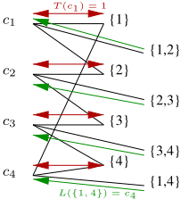
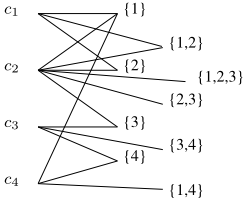
(2020). A witness w will then uniquely identify a concept c if the only edge incident to w is cw.
This demand seemed too strict, and other models where lower complexity could be achieved were considered. However, it became paramount to avoid cheating. In 1996 Goldman and Mathias proposed that a model was collusion-free if further consistent evidence did not make the learner change its mind, i.e., if L(T (c)) = c then for any superset w′ of T (c), if cw′ is an edge of the consistency graph then L(w′ ) = c.
Consider Figure 2 (left); under the classical setting where the only shared information is the consistency graph on black edges, we have minimal GM-collusion-free teaching dimension (NCTD = 1) by the teacher function corresponding to the red matching saturating the concepts. However, TD=1 cannot be achieved with a learner based on concept preferences only, as there is a long cycle for the singletons and we thus have CTD = PBTD = 2. Note that if we add c2 |= 1 and the edges c2{1} and c2{1, 2} and c2{1, 2, 3} to the consistency graph (Figure 2 right) then NCTD = 2. In particular, the red matching is no longer GM-collusion-free, as w = {1, 2} is a superset of both T (c1) and T (c2).
Kirpatrick et al in [2019] proved a theorem stating that a teacher function allows for GM-collusion-free teaching if and only if the consistency graph does not have any induced cycle on 4 edges with 2 of them being chosen by the teacher (as would happen in Figure 2 right, if the red edges in left are chosen by the teacher). They called such a teaching protocol non-clashing and one could view it, in retrospect, as an alternative definition for a GM-collusion-free model of teaching.
In preference-based teaching (PBT) the unique identification rule is relaxed so that the learner will identify c from w, i.e. L(w) = c, as long as w has no edge in the consistency graph to any concept c′ with higher preference than c. It is easy to see that for any teacher and learner adhering to this rule the resulting protocol is GM-collusion-free, as for any node w′ representing a superset of w, the neighbours of w′ will be a subset of the neighbours of w, so if T(c) = w and L(w) = c then also L(w′ ) = c. Note that PBT is a weaker protocol than NCTD, as we see in Figure 2 (left).
Somewhat in parallel with this evolution of consistencybased teaching, there have been some other views of machine teaching, from cases where experiments with humans are performed [Khan et al., 2011] to the use of machine teaching for explainable AI [Yang et al., 2021]. In this case, the teacher selects examples that maximise the explainee's probability of a correct inference. A teaching framework aimed at Bayesian learners is introduced in [Zhu, 2013]. The framework is expressed as an optimisation problem over batch teaching examples that balance the future loss of the learner and the effort of the teacher. A new conceptualisation of expected teaching dimension using a learning and a sampling prior is presented in [Hern´andez-Orallo and Telle, 2020]. Shafto et al. [2014] present the idea that learning can be modelled as Bayesian inference, selecting a small subset of the data that will, with high probability, lead a learner model to the correct inference. A general framework for selecting examples to teach probabilistic learners is presented in [Eaves-Jr. and Shafto, 2016]. Yang and Shafto [2017] use a Bayesian approach where teacher and learner interact and converge on the likelihood of the data given the model on the teacher's side and the posterior of the model given the data on the learner's side inspired by iterative teaching [Liu et al., 2017]. Overall, these papers present an interactive, non-batch setting, do not consider the notion of teaching or do not calculate teaching dimensions. In the traditional machine teaching setting we follow, we assume that the teacher works in a batch mode and sends a witness (e.g., a set of examples) once and for all. Even our use of the term 'changing mind' is metaphorical, as the examples do not come incrementally.
In this paper we study probabilistic teaching models, where the teacher and learner share a generalisation of the consistency graph (which is based on the binary function |= on pairs of concepts and ground elements, which derives into a binary function |= on pairs of concepts and witnesses) in the form of a joint probability distribution of concepts and witnesses p : C ×W → [0, 1]. In this paper we consider only finite concept classes. Even if probabilities could be exploited by teacher and learner to extract confidence in the identification or set different thresholds for p(c|w), in this paper we will require unique identification. This reduces to following p, and since p(c|w) = p(c, w)/p(w) this means:
where arg!max only returns an element if it is unique, otherwise L(w) is undefined (recall that L is a partial mapping). Now, for the teacher, following p means that if T(c) = w we must have p(c|w) > p(c′ |w) for all concepts c′ ̸= c, as the teacher assumes that the learner simply follows the posterior and can identify one concept uniquely with it.
3 MTModels as Witness Joint Distributions
The extension of the consistency graph into a joint distribution assumes that if c and w are inconsistent then p(c, w) = 0, but if c and w are consistent, then p(c, w) > 0 could take any possible value, provided, of course, it is well-defined, i.e., ∑c∈C,w∈W p(c,w) = 1. Basically, the extension converts possibility into probability. The learner then follows:
Table 1 shows a summary of possible cases, depending on the constraints on p(w|c) and p(c) to build estimators for p(c|w). By uniform prior we mean ∀c, c′ : p(c) = p(c′ ). By uniform likelihood we mean ∀c,w,w′ , c |= w, c |= w′ : p(w|c) = p(w′ |c). Note that if w and c are inconsistent then p(w|c) = 0 because p(w, c) = 0. We define the coverage of c as Wc = {w : c |= w}. If this set is finite, then p(w|c) = 1 |Wc| .
When both the likelihood and concept prior are considered uniform we have a few situations already. The general case is actually a new machine teaching model, when coverage sizes |Wc| differ between concepts. Only if the coverage size |Wc| is the same for all c, then we have the extreme case ∀c, c′ ,w,w′ , c |= w, c′ |= w′ : p(w|c) = p(w′ |c′ ). This happens in some well-studied situations, such as any class of Boolean concepts when using both positive and negative examples, since then for any concept c and any w ⊆ 2X there is a unique assignment of negative and positive to elements of w that will be consistent with c. This case really corresponds to the classical teaching (CT) dimension model of Goldman and Kearns [1995]: no preference exists between posteriors and the learner is undefined unless there is unique consistency. If the coverage size is not equal, then the likelihood is higher the smaller the coverage of the concept is, and this would be a specific case of the preference-based teaching (PBT) model of [Gao et al., 2017b; Mansouri et al., 2019], with smaller concepts (in coverage) having preference.
When only the likelihood is assumed uniform we are in a situation that follows the concept prior p(c) and the coverage size of the concept when choosing among several consistent hypotheses. Again, if coverage sizes are equal, we are clearly in the PBT model again, with the priors leading directly to the preferences. However, if coverage sizes are not equal, we can still have an equivalent PBT model that follows the priors by choosing them in an extreme way such that the effect of the likelihood does not affect the choice from the posterior 1 . For instance, Occam's razor, which selects the simpler one of any two consistent hypotheses, could be represented in this way.
When only the concept prior is assumed uniform we are in a situation where the "maximum likelihood estimation" (MLE) is used. Finally, in the general case where both the likelihood and concept prior can vary, we are in the most general case, "maximum a posteriori" (MAP) estimation.
For the two first rows in Table 1, but not the following two rows, we have that they are GM-collusion-free.
Proposition 1. If likelihood is uniform then a learner L based on the posteriors is GM-collusion-free. 2
The notion of GM-collusion-freeness is related to the intuitive principle that increasing consistent evidence should reinforce our beliefs. In a non-probabilistic setting, this is understood as not changing mind for any superset, but this is too extreme an interpretation. A more natural interpretation, which we call the monotonicity property, is that the more examples a learner is given that are consistent with a concept, the more plausibility the learner should assign to that concept, as it rules out other concepts. However, in a probabilistic setting, the probability for a concept c1 can still increase (or not decrease) but another competing concept c2 can increase its probability more, now beating the first. We can translate the monotonicity property to our probabilistic setting as follows. We say that p is monotone iff:
1 We would have to choose a ratio in the priors so high to beat any effect of the likelihoods, i.e, ∀c, c′ , if p(c) > p(c′ ) then p(c)/p(c′ ) > k such that k is greater than any likelihood involving these two concepts.
2 Proofs can be found in https://m.riunet.upv.es/handle/10251/ 182361.
Note that the above property and the definition of GMcollusion-free are very similar. For the two first rows in Table 1 we show that monotonicity is preserved, but this does not hold for the last two rows.
Proposition 2. If likelihood is uniform then p is monotone.
To see why we need to go beyond the first two rows of Table 1, we show in Table 2 an example where changing mind is not necessarily cheating (even if not GM-collusion-free). This is a situation where neither p(w|c) nor p(c) are uniform, but a similar example can be found with p(c) uniform.
We turn to proving results for the last two rows of Table 1, and show that the degree of freedom they allow is very high. We start by defining the minimum teaching dimensions achievable for these new paradigms when likelihoods can be freely chosen (MLE and MAP teaching).
Definition 1. For C on ground elements X, let JDTD +(C) be the lowest teaching dimension achievable by any teacher and learner protocol following a Joint Distribution p : C × 2X . By JDTD ++(C) we denote the analogous quantity for p : C × X∗ , i.e. multisets. We may also require that p is FLUP (free likelihood but uniform prior).
Note JDTD + ≤ JDTD ++ as the former is choosing from a set of witness objects that is a strict subset of the latter. How powerful are these new paradigms? Does the use of any joint distribution p that is restricted only by p(c,w) > 0 ⇔ c |= w allow us to reach the minimum possible teaching dimension in all situations? The answer is Yes. We first define a theoretical lower bound on teaching dimension.
Definition 2. For C on ground elements X and witness set W, and positive integer k, let Gk (C) be the bipartite graph with a vertex for each concept c ∈ C and a vertex for each w ∈ W of at most k > 0 elements from X, and with an edge cw whenever c |= w. Define LBTD +(C) (for W = 2X , i.e. sets) and LBTD ++(C) (for W = X∗ , i.e. multisets), as the minimum k such that Gk (C) has a matching saturating C.
For any teacher mapping T where c |= T (c) we have these variants of LBTD(C) being a Lower Bound on the Teaching Dimension k achieved by T, as the edges {cT(c)}c∈C will form a matching saturating C in the graph Gk (C).
Proposition 3. JDTD + = LBTD + and JDTD ++ = LBTD ++, even for FLUP distributions. For any concept class C on positive examples, with or without repetitions, there is a FLUP joint distribution p such that a learner acting on posteriors achieves lowest possible teaching dimension.
| Case | Existing and New Specific MT Models | p(w|c) | p(c) | Results |
|---|---|---|---|---|
| ULUP - All uniform | CT [Goldman and Kearns, 1995] (concepts with same coverage), PBT [Gao et al., 2017b] (concepts with smaller coverage prevail) | Uniform | Uniform | Monotone and GM- collusion-free |
| ULFP - Uniform Likelihood | PBT [Gao et al., 2017b] and Learning Prior [Hern´andez-Orallo and Telle, 2020] (if all concepts same coverage or extreme priors) | Uniform | Free | Monotone and GM- collusion-free |
| FLUP - Uniform Prior | MLE Teaching | Free | Uniform | Lower bound on TD |
| FLFP - All free | MAP Teaching | Free | Free | Lower bound on TD |
| Concept | p(c) | p(c, ∅) | p(c, {3}) | p(c, {3, 11}) | ... |
| ceven | 0.35 | 0.15 | 0 | 0 | ... |
|---|---|---|---|---|---|
| codd | 0.35 | 0.15 | 0.022 | 0.004 | ... |
| cpow3 | 0.1 | 0.08 | 0.013 | 0 | ... |
| cprime | 0.2 | 0.125 | 0.013 | 0.005 | ... |
We have seen that for the two new machine teaching paradigms MLE and MAP in Table 1, and any Boolean concept class, the theoretically lowest possible TD can be achieved by cherry picking the joint distribution. While it may be the case that these arbitrary distributions are actually the true information about the world that teacher and learner share, for an external observer this is impossible to tell. In order to clarify this, we now take a step back and define a class of joint distributions over witness sets that are FLUP and FF but where the distribution is constructed in a meaningful way.
4 TheWitness Sampling CompositionModel
The original notion of consistency is defined between concepts in C and ground elements in X. As we said at the beginning of section 2, if c is consistent with x1 and x2 then c must be consistent with {x1, x2}. Inconsistencies are also extended from X to W. So, does it make sense that p, the witness joint distribution, is not an extension of the ground joint distribution q? For instance, if q(c, x1) < q(c′ , x1) and q(c, x2) < q(c′ , x2), could p(c, {x1, x2}) > p(c′ , {x1, x2})?
In order to derive p : C ×W → [0, 1] from q : C ×X → [0, 1], we are going to assume that when two or more elements in X are composed in W their composition is performed as a sampling process. We call this assumption Witness Sampling Composition (WSC), and we define it as follows: WSC means that the construction of witnesses is modelled as a sampling procedure from X where the extraction of one element does not affect the relative probabilities of extracting the remaining elements (with or without replacement). We define the WSC construction of p from q recursively, with the base case given by p(c, λ) = r(0) · q(c) where λ represents the empty witness (no example has been sampled yet) and r is a regularisation term (with ∑n r(n) = 1) we will explain later. The recursive step is defined as follows:
| Concept | q(c) | q(c, 3) | q(c, 11) | ... |
| ceven | 0.35 | 0 | 0 | ... |
|---|---|---|---|---|
| codd | 0.35 | 0.087 | 0.0054 | ... |
| cpow3 | 0.1 | 0.05 | 0 | ... |
| cprime | 0.2 | 0.05 | 0.0062 | ... |
where |w| represents the dimension of w (number of elements in w), and w = w′ ⊕xi represents that witness w is composed of a smaller witness w′ (of dimension |w| - 1) and xi ∈ X. Finally, with x ∈ X-w′ we denote any x that can be sampled from X after w′ has been sampled (with replacement or not). Note the difference between the first and second line of the previous derivation is just a normalisation keeping the proportions (which is q(c) when there is replacement).
Proposition 4. Under WSC, the concept priors are preserved between q and p, i.e.: ∀c ∈ C : p(c) = q(c)
The meaning of the regularisation term r comes from the fact that ∀c ∀n ≥ 0 : ∑w∈W:|w|=n p(c,w) = r(n) · q(c) but, as q(c) = p(c) = ∑w∈W p(c,w), then r is actually a regularisation probability r : N → [0, 1], where r(n) represents how likely all the witnesses of dimension n are. In other words, if we are given the ground joint distribution q, expressing how likely any pair of concept and witness is, and we are also given how likely each dimension is, then we can derive the witness joint distribution. The choice of r does not affect the behaviour of the learner (arg!maxc p(c|w)), as when w is given, we have the same r(|w|) for all concepts.
We give two examples of ground distributions q and the resulting WSC derived witness distributions p. One for subsets of natural numbers and sampling without replacement, with q in Table 3 and p in Table 2, and one example with coins illustrating sampling with replacement in Table 4.
| Concept | p(c) | q(c,H) | q(c, T) | p(c, {H}) | p(c, {T}) | p(c, {HT}) | p(c, {HTT}) |
| coin1 | 0.25 | 0.2 | 0.05 | 0.05 | 0.0125 | 0.005 | 0.0005 |
| coin2 | 0.25 | 0.125 | 0.125 | 0.031 | 0.031 | 0.0078 | 0.0020 |
| coin3 | 0.25 | 0.10 | 0.15 | 0.025 | 0.037 | 0.007 | 0.00225 |
| coin4 | 0.25 | 0.05 | 0.2 | 0.0125 | 0.05 | 0.005 | 0.0020 |
5 Teaching Dimension of theWSCModel
This section shows the remaining inequalities in Figure 1.
Definition 3. For C over ground elements X, let WSCTD +(C) be lowest teaching dimension achievable by p : C×2X derived by WSC from joint distribution q : C×X, with WSCTD ++(C) the analogous for p : C ×X∗ .
We start with the case of sets. First, is WSC a real restriction over the free case in Table 1? We can answer this in the affirmative with a simple proof.
Our next result shows that WSCTD +, even when restricted to FLUP distributions, is as powerful as any nonclashing teaching model. To prove this proposition we construct a ground joint distribution that cherry-picks the nonclashing teacher function, by assigning small values to q(c, x) if c |= x but x ̸∈ T(c). Note however that these values are not exponentially small, as they satisfy q(c, x) > 1/|C|3 .
Proposition 6. WSCTD + ≤ NCTD +. For any C we have a FLUP distribution q : C ×X such that p : C × 2X derived by WSC from q shows that WSCTD +(C) ≤ NCTD +(C).
Now we turn to the set of witness objects being multisets over X. Firstly, as in the set case, there is an easy proof showing that WSC ++ is not as free as JDTD ++.
This proof actually shows that WSCTD avoids a very unnatural situation which looks like cheating, e.g. tossing a coin where Tail is more likely than Head but two Heads more likely than two Tails, and this is forbidden by WSCTD. Finally, we show a somewhat surprising result comparing teaching dimensions using witness objects that are multisets versus sets, showing that WSCTD ++ restricted to FLUP distributions will achieve the theoretical lower bound LBTD +. To prove this proposition we construct a ground joint distribution that cherry-picks any given matching in Gk (C) as per Definition 2, by assigning small values to q(c, x) if c |= x but x ̸∈ T (c). These values satisfy q(c, x) > 1/(|C||X|)2 .
Proposition 8. WSCTD ++ ≤ LBTD + = JDTD +. For any concept class C over X and set of witness objects W = 2X , there exists a FLUP joint distribution q : C × X such that p : C×X∗ derived by WSC with replacement from q has teaching dimension LBTD +(C) = JDTD +.
6 Discussion
[Kirkpatrick et al., 2019] was a remarkable paper clarifying the limits of the classical view of cheating as GM-collusion, by reinterpreting it as non-clash machine teaching. This seemed the culmination of over twenty years work of finding more and more powerful GM-collusion-free models, i.e., the most powerful non-cheating teaching models. However, we have challenged this very notion of cheating, under a natural probabilistic view. The notion of full-proof identification is replaced by the inductive notion of a guess, and the learners can 'change their mind' as posteriors are affected by changing likelihoods. We have also shown that in some particular cases (e.g., dealing with the empty set), the GM-collusionfree paradigm can allow some unnatural assignments.
The use of a witness joint probability p has been shown powerful enough to equal the best achievable teaching dimension, LBTD, and in some cases, it can also do some unnatural assignments. Instead, we have proposed to derive p from the ground joint distribution q using WSC, in the same way as the consistency graph for witnesses derives from the consistency graph for ground elements, depending on how witnesses are composed. The new teaching models deriving from WSC are shown to be slightly less powerful than LBTD, but avoid the unnatural situations. As a result, whether a teacher and learner do any cheating depends on whether the ground joint distribution corresponds to the joint beliefs about the world. If a teacher and learner know that a coin has 73% bias for heads, using this information for identifying the coin is not cheating. Cheating would be if both agreed that this coin had a different bias from the actual, one more convenient for the identification. We see a promising avenue of future work on the analysis of how much information teacher and learner share by fixing the entropy of the joint distributions and thinking of the distribution of this entropy that reduces the uncertainty of the identification. Also, we could pursue the idea that some choices of r could lead to a likelihood that is guiding the teacher, as in Bayesian teaching.
The general and refreshing probabilistic perspective synthesised in Table 1, and the connections with the classical teaching models, suggest that our paper could help bridge two very different conceptions of machine teaching in AI. There is the classical notion of identification, associated with theoretical results about the teaching dimension, and a more modern view of machine teaching as a probabilistic (or Bayesian) process. This should lead to future work connecting our schema to areas such as MDL/MML [Wallace and Dowe, 1999] inference, or when teacher and learner can adapt their probabilities. All this can be explored with a more natural paradigm of non-cheating teaching that allows changes of mind.
Acknowledgments
We would like to thank Pekka Parviainen for providing insights that led to the witness sampling composition. We thank the anonymous reviewers for their comments and interaction during the discussion process. This work has been partially supported by the Norwegian Research Council grant 329745 Machine Teaching for Explainable AI, also by the EU (FEDER) and Spanish MINECO grant RTI2018-094403-BC32 funded by MCIN/AEI/10.13039/501100011033 and by "ERDF A way of making Europe", Generalitat Valenciana under grant PROMETEO/2019/098, EU's Horizon 2020 research and innovation programme under grant agreement No. 952215 (TAILOR), and INNEST/2021/317 (Project cofunded by the European Union with the "Programa Operativo del Fondo Europeo de Desarrollo Regional (FEDER) de la Comunitat Valenciana 2014-2020").
@inproceedings{ijcai2022p412,
  title     = {Non-Cheating Teaching Revisited: A New Probabilistic Machine Teaching Model},
  author    = {Ferri, Cèsar and Hernández-Orallo, José and Telle, Jan Arne},
  booktitle = {Proceedings of the Thirty-First International Joint Conference on
               Artificial Intelligence, {IJCAI-22}},
  publisher = {International Joint Conferences on Artificial Intelligence Organization},
  editor    = {Luc De Raedt},
  pages     = {2973--2979},
  year      = {2022},
  month     = {7},
  note      = {Main Track},
  doi       = {10.24963/ijcai.2022/412},
  url       = {https://doi.org/10.24963/ijcai.2022/412},
}
TY - CPAPER TI - Non-Cheating Teaching Revisited: A New Probabilistic Machine Teaching Model AU - Ferri, Cèsar AU - Hernández-Orallo, José AU - Telle, Jan Arne T2 - Proceedings of the Thirty-First International Joint Conference on Artificial Intelligence, IJCAI-22 PB - International Joint Conferences on Artificial Intelligence Organization PY - 2022 SP - 2973 EP - 2979 DO - 10.24963/ijcai.2022/412 UR - https://doi.org/10.24963/ijcai.2022/412 ER -Copied
Machine-readable versions of this paper, for tools and AI agents:





