
A Reinforcement Learning-Informed Pattern Mining Framework for Multivariate Time Series Classification
Proceedings of the Thirty-First International Joint Conference on Artificial Intelligence. Main Track. Pages 2994-3000.
https://doi.org/10.24963/ijcai.2022/415
Keywords
- Multidisciplinary Topics and Applications: Health and Medicine
- Machine Learning: Classification
- Machine Learning: Deep Reinforcement Learning
- Machine Learning: Time-series; Data Streams
Abstract
Multivariate time series (MTS) classification is a challenging and important task in various domains and real-world applications. Much of prior work on MTS can be roughly divided into neural network (NN)- and pattern-based methods. The former can lead to robust classification performance, but many of the generated patterns are challenging to interpret; while the latter often produce interpretable patterns that may not be helpful for the classification task. In this work, we propose a reinforcement learning (RL) informed PAttern Mining framework (RLPAM) to identify interpretable yet important patterns for MTS classification. Our framework has been validated by 30 benchmark datasets as well as real-world large-scale electronic health records (EHRs) for an extremely challenging task: sepsis shock early prediction. We show that RLPAM outperforms the state-of-the-art NN-based methods on 14 out of 30 datasets as well as on the EHRs. Finally, we show how RL informed patterns can be interpretable and can improve our understanding of septic shock progression.
- [Anzai, 2012] Yuichiro Anzai. Pattern recognition and machine learning. Elsevier, 2012.
- [Bagnall et al., 2018] Anthony Bagnall, Hoang Anh Dau, Jason Lines, Michael Flynn, James Large, Aaron Bostrom, Paul Southam, and Eamonn Keogh. The uea multivariate time series classification archive. arXiv preprint arXiv:1811.00075, 2018.
- [Dempster et al., 2020] Angus Dempster, Franc ¸ois Petitjean, and Geoffrey I Webb. Rocket: exceptionally fast and accurate time series classification using random convolutional kernels. Data Mining and Knowledge Discovery, 34(5):1454-1495, 2020.
- [Dempster et al., 2021] Angus Dempster, Daniel F Schmidt, and Geoffrey I Webb. Minirocket: A very fast (almost) determin- istic transform for time series classification. In Proceedings of the 27th ACM SIGKDD Conference on Knowledge Discovery & Data Mining, pages 248-257, 2021.
- [Demšar, 2006] Janez Demšar. Statistical comparisons of classifiers over multiple data sets. JMLR, 7:1-30, 2006.
- [Dulac-Arnold et al., 2015] Gabriel Dulac-Arnold, Richard Evans, Hado van Hasselt, Peter Sunehag, Timothy Lillicrap, Jonathan Hunt, Timothy Mann, Theophane Weber, Thomas Degris, and Ben Coppin. Deep reinforcement learning in large discrete action spaces. arXiv preprint arXiv:1512.07679, 2015.
- [Gao et al., 2021] Ge Gao, Samiha Marwan, and Thomas W Price. Early performance prediction using interpretable patterns in pro- gramming process data. In Proceedings of the 52nd ACM Techni- cal Symposium on Computer Science Education, pages 342-348, 2021.
- [Gao et al., 2022a] Ge Gao, Farzaneh Khoshnevisan, and Min Chi. Reconstructing missing ehrs using time-aware within-and cross- visit information for septic shock early prediction. ICHI, 2022.
- [Gao et al., 2022b] Qitong Gao, Dong Wang, Joshua D Amason, Siyang Yuan, Chenyang Tao, Ricardo Henao, Majda Hadziahme- tovic, Lawrence Carin, and Miroslav Pajic. Gradient importance learning for incomplete observations. ICLR, 2022.
- [Hallac et al., 2017] David Hallac, Sagar Vare, Stephen Boyd, and Jure Leskovec. Toeplitz inverse covariance-based clustering of multivariate time series data. In ACM SIGKDD Int. Conf. on Knowledge Discovery and Data Mining, pages 215-223, 2017. IJCAI
- [Hochreiter and Schmidhuber, 1997] Sepp Hochreiter and Jürgen Schmidhuber. Long short-term memory. Neural computation, 9(8):1735-1780, 1997.
- [Holm, 1979] Sture Holm. A simple sequentially rejective multiple test procedure. Scandinavian journal of statistics, pages 65-70, 1979.
- [Johnson et al., 2016] Alistair EW Johnson, Tom J Pollard, Lu Shen, H Lehman Li-Wei, Mengling Feng, Mohammad Ghas- semi, Benjamin Moody, Peter Szolovits, Leo Anthony Celi, and Roger G Mark. Mimic-iii, a freely accessible critical care database. Scientific data, 3(1):1-9, 2016.
- [Kang and Choi, 2014] Hyohyeong Kang and Seungjin Choi. Bayesian common spatial patterns for multi-subject eeg classi- fication. Neural Networks, 57:39-50, 2014.
- [Karim et al., 2019] Fazle Karim, Somshubra Majumdar, Houshang Darabi, and Samuel Harford. Multivariate lstm-fcns for time series classification. Neural Networks, 116:237-245, 2019.
- [Keogh and Lin, 2005] Eamonn Keogh and Jessica Lin. Clustering of time-series subsequences is meaningless: implications for pre- vious and future research. Knowledge and information systems, 8(2):154-177, 2005.
- [Le Nguyen et al., 2019] Thach Le Nguyen, Severin Gsponer, Iulia Ilie, Martin O'Reilly, and Georgiana Ifrim. Interpretable time se- ries classification using linear models and multi-resolution multi- domain symbolic representations. Data mining and knowledge discovery, 33(4):1183-1222, 2019.
- [Li et al., 2021] Guozhong Li, Byron Choi, Jianliang Xu, et al. Shapenet: A shapelet-neural network approach for multivariate time series classification. In AAAI, volume 35, pages 8375-8383, 2021.
- [Lillicrap et al., 2016] Timothy P Lillicrap, Jonathan J Hunt, Alexander Pritzel, et al. Continuous control with deep reinforce- ment learning. ICLR, 2016.
- [Lloyd, 1982] Stuart Lloyd. Least squares quantization in pcm. IEEE Tran. on Info. Theory, 28(2):129-137, 1982.
- [Minnen et al., 2006] David Minnen, Thad Starner, et al. Discover- ing characteristic actions from on-body sensor data. In 2006 10th IEEE international symposium on wearable computers, pages 11-18. IEEE, 2006.
- [Rakthanmanon and Keogh, 2013] Thanawin Rakthanmanon and Eamonn Keogh. Fast shapelets: A scalable algorithm for dis- covering time series shapelets. In SDM, pages 668-676. SIAM, 2013.
- [Ruder, 2016] Sebastian Ruder. An overview of gradient descent optimization algorithms. arXiv preprint arXiv:1609.04747, 2016.
- [Ruiz et al., 2021] Alejandro Pasos Ruiz, Michael Flynn, James Large, Matthew Middlehurst, and Anthony Bagnall. The great multivariate time series classification bake off: a review and ex- perimental evaluation of recent algorithmic advances. Data Min- ing and Knowledge Discovery, 35(2):401-449, 2021.
- [Schäfer and Leser, 2018] Patrick Schäfer and Ulf Leser. Multivari- ate time series classification with weasel+ muse. arXiv, 2018.
- [Senin and Malinchik, 2013] Pavel Senin and Sergey Malinchik. Sax-vsm: Interpretable time series classification using sax and vector space model. In ICDM, pages 1175-1180. IEEE, 2013.
- [Shokoohi-Yekta et al., 2015] Mohammad Shokoohi-Yekta, Jun Wang, and Eamonn Keogh. On the non-trivial generalization of dynamic time warping to the multi-dimensional case. In SDM, pages 289-297. SIAM, 2015.
- [Tan et al., 2016] Pang-Ning Tan, Michael Steinbach, and Vipin Kumar. Introduction to data mining. Pearson Education India, 2016.
- [Yang et al., 2021] Xi Yang, Yuan Zhang, and Min Chi. Multi- series time-aware sequence partitioning for disease progression modeling. In IJCAI, 2021.
- [Ye and Keogh, 2009] Lexiang Ye and Eamonn Keogh. Time series shapelets: a new primitive for data mining. In ACM SIGKDD Int. Conf. on Knowledge discovery and data mining, pages 947-956, 2009.
- [Zhang et al., 2020] Xuchao Zhang, Yifeng Gao, Jessica Lin, and Chang-Tien Lu. Tapnet: Multivariate time series classification with attentional prototypical network. In AAAI, volume 34, pages 6845-6852, 2020.
- [Zoph and Le, 2017] Barret Zoph and Quoc V Le. Neural architec- ture search with reinforcement learning. ICLR, 2017.
References were extracted automatically from the PDF and may contain errors.
Full text extracted automatically from the PDF; figures, tables and equations may differ. The PDF is the version of record.
1 Introduction
Multivariate time series (MTS) are sequences of events acquired longitudinally, where each event is constituted by observations recorded over multiple attributes. For example, the vital signs and lab results in electronic health records (EHRs) can be formulated as MTS, since they are measured over time and multiple measurements can be obtained simultaneously (e.g., temperature and blood pressure). MTS are widely used in motion recognition [Rakthanmanon and Keogh, 2013], human activity recognition [Minnen et al., 2006], and healthcare [Kang and Choi, 2014]. Comprehensive analyses of MTS can provide insights and facilitate decision-making in various domains and applications [Senin and Malinchik, 2013], and MTS classification is one of the fundamental problems of MTS analyses and has received significant attention [Li et al., 2021]. In general, previous work on MTS classification can be roughly divided into the more recent, highly effective neural network (NN)- based methods, and the classic, often interpretable pattern-based methods.
Various NN-based approaches have been proposed to directly learn low-dimensional representations from MTS through various NN or deep NNs, including the state-of-theart ROCKET [Dempster et al., 2020], TapNet [Zhang et al., 2020], and MLSTM-FCN [Karim et al., 2019]. For example, ROCKET uses a large number of random convolution kernels to transform time series and uses the transformed representations to train a linear classifier. Despite their effectiveness, due to the 'black-box' nature of neural network models, the learned representations are often hard to interpret.
The pattern-based methods, on the other hand, generate discrete representations or time-series shapelet as patterns that capture both intra- and inter-sample structures of MTS (e.g., ShapeNet [Li et al., 2021], WEASEL+MUSE [Sch¨afer and Leser, 2018]). These methods decompose each original attribute into a bag of substructures using sliding windows, then transform the substructures into features to be used as inputs for classifiers. Since the patterns are still operating on the original attribute space, they are often highly interpretable. Specifically, discriminative patterns are those that can distinguishMST among different classes [Senin andMalinchik, 2013] and they are typically useful for classification tasks. As frontier work, WEASEL+MUSE [Sch¨afer and Leser, 2018] applies symbolic Fourier approximation to discretize MTS and uses χ2 -test to determine discriminative patterns.
In addition to the fact that pattern-based methods often produce interpretable patterns which may not be helpful for classification, they also have three major limitations: (i) Generalizability - to determine discriminative patterns, pattern-based methods typically use carefully designed architectures, often in combination with domain knowledge over specific types of data [Gao et al., 2021]. (ii) Scalability - they tend to generate a great amount of pattern candidates and require complicated feature filtering modules. This could lead to inefficient training and undesirable model performance as discussed in [Zhang et al., 2020]. (iii) Reliability - existing patternbased methods employ distance-based metrics, i.e. dynamic time warping (DTW) [Shokoohi-Yekta et al., 2015] and symbolic Fourier approximation [Sch¨afer and Leser, 2018] to discretize and segment MTS,. Yet, these are not considered to be very reliable [Hallac et al., 2017].
We propose a Reinforcement Learning (RL) informed PAttern Mining (RLPAM) framework to identify interpretable yet important patterns for MTS classification.
| Used as baselines | ||||||||
|---|---|---|---|---|---|---|---|---|
| Method | DTW | WEASEL +MUSE (2018) | MLSTM -FCN (2019) | TapNet (2020) | ShapeNet (2021) | ROCKET (2020) | # of UEA datasets | Wins |
| WEASEL+MUSE MLSTM-FCN TapNet | ✓ ✓ ✓ ✓ ✓ | ✓ ✓ ✓ ✓ | ✓ | ✓ ✓ ✓ | ✓ | 20 20 30 30 26 | 13 14 14 14 9 | |
| ✓ | ||||||||
| ShapeNet ROCKET | ✓ | |||||||
| RLPAM (Ours) | ✓ | ✓ | ✓ | 30 | 16 | |||
RLPAM combines Deep RL (DRL) and Toeplitz inverse covariance-based clustering (TICC) to address limitations and shortcomings of existing pattern-based approaches while preserving their original interpretability. DRL have shown great success in improving prediction performance [Gao et al., 2022b; Zoph and Le, 2017], which do not necessarily rely on domain knowledge. By considering the graphical connectivity structure of both the temporal and the crossattribute dependencies among events, it has been shown that TICC produces more reliable results in MTS segmentation than distance-based metrics, as well as discovering pattern interpretations in various applications such as driving patterns in traffic [Hallac et al., 2017; Yang et al., 2021].
We compare RLPAM with other the-state-of-the-art NNbased and pattern-based methods on 30 benchmark datasets as shown in Table 1 as well as real-world large-scale EHRs for a challenging task: sepsis shock early prediction. RLPAM outperforms all other methods on 14 out of 30 datasets as well as on the EHRs. We also show that by selecting patterns based on RL, not only can the performance of classification be improved, but they can also be used to draw insights into quantitative and qualitative relationships between MTS and labels through a case study using the task of septic shock progression. To summarize, our work has at least two main contributions: 1) To the best of our knowledge, RLPAM is the first MTS classification method to adapt RL to identify discriminative patterns, making the framework scalable, generalizable, and reliable; 2) We have conducted a comprehensive comparison of various state-of-the-art NN-based and patternbased methods across 30 UEA Archive datasets (Table 1).
2 RelatedWork
Table 1 summarizes the performance of some recently proposed MTS classification models comparing with their respective baselines over the UEA datasets. These methods in general can be categorized into pattern-based and NN-based.
Pattern-based methods generally extract bag-of-patterns (BOP) (e.g., WEASEL+MUSE [Sch¨afer and Leser, 2018]) or shapelet-patterns (e.g., ShapeNet [Li et al., 2021]) from time series and then feed these patterns into a classifier. Specifically, BOP breaks up time series into windows and represents them as discrete features via a histogram of feature counts. For instance, one of the state-of-the-art BOP models, WEASEL+MUSE [Sch¨afer and Leser, 2018], uses symbolic Fourier approximation and statistical methods to generate discrete-valued patterns for classification. It outperforms classic baselines (e.g., DTW) on 13 out of 20 UEA datasets. Shapelets are time series subsequences that can best represent samples across different classes [Ye and Keogh, 2009].
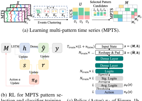
lection and classifier training. (c) Policy (Actor) πθ of Figure 1b.
Figure 1: Overview of the RLPAM framework.
ShapeNet [Li et al., 2021] embeds shapelets into a unified space and characterizes MTS by evaluating pre-defined distance metrics calculated from selected shapelets as inputs to the classification model. It outperforms baselines including WEASEL+MUSE on 14 out of 30 UEA datasets.
NN-based methods [Karimet al., 2019; Zhang et al., 2020] have been proposed to improve the MTS classification performance recently. For instance, MLSTM-FCN [Karim et al., 2019] is a deep learning framework that generates latent patterns with a squeeze-and-excitation block, and it outperforms WEASEL+MUSE on 14 out of 20 UEA datasets. TapNet [Zhang et al., 2020] proposes an attentional prototype network to learn the latent features extracted fromMTS, and it outperforms both benchmark and recent baselines (e.g., MLSTM-FCN) on 14 out of 30 UEA datasets. ROCKET [Dempster et al., 2020] is neural-network based model that transforms time series using random convolutional kernels to train linear classifiers. It is recognized as a strong method evaluated on 26 UEA datasets in recent work [Ruiz et al., 2021]. Although these NN-based approaches can be trained end-to-end, they provide little interpretability.
3 RLPAM
The overview of our RLPAM framework is illustrated in Figure 1. It first encodes MTS into univariate cluster sequences (UCS), then learns multi-pattern time series (MPTS) using pattern candidates extracted from UCS, from which discriminative patterns are identified by a RL module, in concurrent with training of the classification model. We are releasing the source code of our implementation and it can be accessed at https://github.com/fay067/RLPAM.
3.1 ProblemFormulation
Multivariate time series can be represented as X = {X1, ...,XN}, where N is the total number of samples. Each sample Xi consists of a sequence of events: Xi = (xi,1, ..., xi,ti ) where each xi,j is an event representing the observations at time step j and ti is the horizon which can vary across different samples. Specifically, xi,j ∈ RD and D is the number of attributes recorded; thus, we have Xi ∈ Rti×D . Our goal is to train a classification model f : Xi → yi which assigns each sample Xi to its corresponding class yi ∈ P = {1, ..., P}.
3.2 LearningMulti-pattern Time Series
Encoding UCS from MTS. We first convert each MTS sample Xi into a univariate cluster sequence (UCS), which is a vector characterizing the dependencies across attributes in the original MTS. It consists of the following two steps: Events Clustering: Events from all samples are stacked to form a multivariate sequence X = (x1,1, ..., x1,t1 , ..., xN,1, ..., xN,tN ) with length T = ∑Ni=1 ti. Then we group the events xi,j ∈ X into C clusters, where each xi,j is assigned with one from the set of clusters K = {K1, . . . , KC}. The distance-based metrics used in classic clustering methods, such as K-Means [Lloyd, 1982], are shown to be not fully reliable for pattern mining purposes [Keogh and Lin, 2005; Hallac et al., 2017]. As a result, we choose to formulate the objective as defined in the Toeplitz inverse covariancebased clustering (TICC) problem [Hallac et al., 2017], since it can be solved through a model-based manner by considering the graphical connectivity structure of both the temporal and the cross-attribute dependencies among events. UCS Formulation: After mapping each event into a cluster, a vector K = (K1,1, . . . ,K1,t1 , . . . ,KN,1, . . . ,KN,tN ) can be defined such that each element Ki,j ∈ K is mapped from the corresponding event xi,j ∈ X. Then we group together the Ki,j's that are mapped from the same sample as Ui = (Ki,1, . . . , Ki,ti ) to constitute the UCS for sample Xi.
Extracting MPTS from UCS. From the pattern information encoded in UCS, we further extract multi-pattern time series (MPTS) to represent the time series samples. It consists of the following two steps: Initializing Pattern Candidates: For the set of UCS, Up p ∈ P, which mapped from samples {Xi|yi = p} associated with a class p, we extract consecutive subsequences with a minimum length of 2, as pattern candidates unique to class p. Consequently, the overall set of pattern candidates for all the classes, L = {l1, . . . , lL}, can be obtained by extracting subsequences from all Up and taking a union of their outputs; here, L is the size of such pattern candidates set. Encoding Multi-Pattern Time Series: Given a sample Xi with length ti, its MPTS over L pattern candidates is written as Mi = (Mi,1, ...,Mi,L)⊤ ∈ {0, 1}ti×L, where Mi,l ∈ {0, 1}ti . The elements of Mi,l are determined by the time stamps the l-th pattern candidate appears (denoted as 1) or is absent (denoted as 0) in its corresponding UCS Ui. Note that such MPTS encapsulate the dependencies underlying sequential patterns across timestamps and samples, and they could be used as the inputs to a classification model.
3.3 RL for Pattern Selection and Classification
Considering the fact that the number of MPTS pattern candidates {l1, . . . , lL} are usually large, it is highly desired to filter out the noisy patterns to classify based on critical ones. Though some linear models, e.g., LASSO, may be capable of selecting patterns based off fromMPTS, they cannot capture the temporal correlations existed in MTS [Tan et al., 2016]. In this work, we introduce RL to simplify the MPTS Mi's by identifying the discriminative patterns, which can best distinguish each sample among the classes, by interacting with the RL environment while training the classifier f. Equipped with RL, our method can not only improve the performance of f, but also highlight interpretability of the patterns.
There exists at least two challenges for RL to solve the problem we consider. (a) Large discrete search space. The number of pattern candidates could result in exponentially growing search space since it has size 2L. (b) Sampleagnostic discriminative pattern selection. Usually the classification model is trained using mini-batches which are randomly sampled from the training dataset [Ruder, 2016]. However, we expect the selected discriminative patterns to distinguish each sample among all the others that are not associated with the same class, even if they are not presented in the current training batch. As a result, we expect the RL to select a set of patterns that are consistently discriminative among all the samples, instead of finding patterns that can only distinguish samples within each specific input batch.
Modeling with RL
General RL trains an agent to learn optimal strategies by interacting with environments and maximizing cumulative rewards. Such environments can be formalized as Markov decision processes (MDPs). Specifically, each time after the agent performs an action a = π(s) at state s following its policy π, the environment responds with the next state s′ with the reward signal r. The goal is to find a policy π that maximizes the expected cumulative return the agent could obtain, as G(π) = Eρ [ ∑ητ=0 γ iR(sτ , aτ )]; here, η is the horizon of the environment, ρ = {(s0, a0), . . . , (sη, aη)|aτ = π(sτ )} is the trajectory given π, and γ ∈ [0, 1) is the discount factor.
The modeling of MPTS pattern selection and training an LSTM [Hochreiter and Schmidhuber, 1997] classifier based on RL is illustrated in Figure 1b. Each element of M = (S, A, P, R, γ) in this RL environment is detailed as follows:
State Space S: The states are characterized by s = (M, h), where M ∈ {0, 1}Ttrain×L is the batch of MPTS mapped from corresponding training samples selected in the current iteration, Ttrain = ∑Ntrain i=1 ti, h ∈ RNtrain×nlstm are the encodings (or the hidden states) generated by the LSTM, Ntrain is the batch size and nlstm is the number of hidden units of the LSTM.
Action Space A: The action space defines the mechanism of selecting discriminative patterns from all the L patterns residing within the input batch M. We define actions as vectors with length L as a ∈ {0, 1}L. Each dimension l ∈ [1,L] is filled with either 1 (or 0) corresponding to if the l-th pattern in M is considered as a discriminative pattern (or not).
Given that there exists one-to-one mapping between each Xi and Mi following from Section 3.2, we can rewrite the classification model's input in terms of MPTS under the batch training setting to simplify mathematical notations. Specifically, from now on we consider the classification model f takes as input batch M⊙ a and maps them to predictions ˆy, where M⊙a means all the elements in the l-th column of M
are multiplied with the l-th element in a for all l ∈ [1, L].
Transitions P: The transition dynamics determine how to transit from a current state s = (M, h) to the next state s′ = (M′ , h′ ) given an action a to the environment. In our case, M → M′ is determined by how training batches are formulated by sampling from the dataset in each iteration. Similarly, h → h′ represents the change of LSTM hidden states by switching from the old input M⊙a to the new input M′ ⊙a′ . Consequently, by putting together all the transitions above, we define s → s′ .
Reward Function R: After the agent takes an action a at state s, the reward r = R(s, a) is returned by the environment, thus the policy π can then be updated following this information. We define the reward function as R(s, a) =
-J(ˆy, y), which is the negative of a commonly used loss function such as cross-entropy.
Actor-Critic DRL. Although some existing RL methods can resolve the challenge (a), e.g., [Dulac-Arnold et al., 2015], they may not be capable of addressing the challenge (b), which is specific to the pattern selection problem considered in this work. Here, we choose to adapt from an actorcritic deep RL method, i.e., deep deterministic policy gradient (DDPG) [Lillicrap et al., 2016], for two reasons. First, it was originally designed for continuous action spaces which intrinsically has large spaces; Second, the policy π can be updated using past experience, which is more sampling efficient. In DDPG, an actor πθ : S → A is used to represent the policy to be updated iteratively. It is parametrized by a multi-layer perceptron (MLP) [Anzai, 2012] θ. The actor πθ is jointly trained with the critic Qξ : S × A → R, parametrized by another MLP ξ, to maximize the approximated expected return Gβ(πθ) = Es∼ρβ [Qξ(s, πθ(s))].
Our Neural Architecture and Actor-Critic Updates
We first design the neural architecture for actor πθ to account for the discrete action space a ∈ {0, 1}L, by using Sigmoid output activations and thresholding. The architecture is illustrated by a flowchart in Figure 1c. Specifically, to better represent the states s = (M, h) as matrices in batch settings, we define ˜s = ( ˜M, h) where ˜M is obtained by first padding all the sequences Mi ∈ M to become the same length and then concatenating all the elements in each padded sequence into a vector; thus, the first dimension of ˜Mbecomes Ntrain, which is consistent with h ∈ RNtrain×nlstm . 1 Then, the architecture follows regular MLP up until when logits are generated, which are with dimension RNtrain×L. In what follows, the logits first pass through a Sigmoid layer and are then averaged over all the samples in batch, where we denote the output from here as µθ(s) ∈ RL. At last, the action is generated following πθ(s) = 1(µθ(s) ≥ 0.5), where 1(·) is the indicator function and πθ(s) ∈ RL.
Due to the averaging layer, the same action is taken for all the inputs in the batch, i.e., the same patterns are selected over all the input samples (Xi's) that are mapped to the MPTS batch M. The purpose of using such an averaging layer is to reduce the conditional dependencies between a and s as pointed out in the challenge (b). Since each batch is formed by randomly sampling from the training data, by enforcing such constraints we expect the policy would focus on the patterns that are helpful to distinguish different classes.
1 Note that ˜s and s can be used interchangeably.
Note that the updates of policy πθ do not rely on domain knowledge of the datasets, which shows generalizability of the framework. The use of deep classification models and deep RL makes the proposed method scalable. In event clustering, the objective does not include the distance-based metrics that are shown to be not fully reliable. Moreover, the selected discriminative patterns could be interpretable, which will be illustrated in Section 4.5.
4 Experiments
In this section, we introduce the datasets and baselines used for evaluations, followed by results and a case study illustrating the interpretability of derived patterns.
4.1 Datasets
We first evaluate our model on 30 datasets from UEA MTS classification archive [Bagnall et al., 2018], which consists of data collected from various domains, including human activities recognition, ECG/EEG signals, motion classification, etc. The sample sizes of the datasets range from 27 to 50,000. The lengths of time series range from 8 to 17,901. We follow the same train/test split ratio as provided by the dataset authors.
Furthermore, we evaluate our model's performance on 24-hour early predictions of septic shock using MIMIC-III [Johnson et al., 2016] which contains real-world electronic healthcare records obtained from intensive care unit patients. We pre-process and label sepsis patients following [Gao et al., 2022a]. In total 772 (containing 386 positive and 386 negative) sepsis patients are obtained. The lengths of time series range from 1 to 923. We adopt 5-fold cross validation to evaluate the performance on this dataset.
4.2 EvaluationMetrics
For each dataset, we report the classification accuracy, average rank and number of wins/ties on the testing set. We compute mean per class error (MPCE), which is the average error of each class for all the datasets, following the process described in [Karim et al., 2019]. We also conduct the Friedman test and Wilcoxon signed-rank test following the process described in [Demˇsar, 2006] with Holm's α (5%) [Holm, 1979]. The Friedman test is a non-parametric statistical test to justify the significance of performance differences across all the methods. The Wilcoxon signed-rank test is a non-parametric statistical test based on the hypothesis that the rank medians between our method and any baselines are the same.
4.3 Baselines
We compare RLPAM with (i) directly using UCSs as inputs to train LSTM, which is denoted as UCS in Table 2. This serves as an ablation baseline which helps analyze the advantages of mining discriminative patterns from them, as proposed in RLPAM. (ii) Seven state-of-the-art methods: WEASEL+MUSE, ShapeNet, MLSTM-FCN, TapNet, and ROCKET as reviewed in Section 2, as well as MrSEQL [Le Nguyen et al., 2019] and MiniRocket [Dempster et al., 2021], which are originally
| Dataset | EDI | DTWI | DTWD | WEASEL +MUSE (2018) | MLSTM -FCN (2019) | MrSEQL (2019) | TapNet (2020) | ShapeNet (2021) | ROCKET (2020) | MiniRocket (2021) | UCS | RLPAM |
|---|---|---|---|---|---|---|---|---|---|---|---|---|
| AF | 0.267 | 0.267 | 0.200 | 0.333 | 0.267 | 0.267 | 0.333 | 0.400 | 0.067 | 0.133 | 0.467 | 0.733 |
| HMD | 0.279 | 0.306 | 0.231 | 0.365 | 0.365 | 0.149 | 0.378 | 0.338 | 0.446 | 0.392 | 0.432 | 0.635 |
| SWJ | 0.200 | 0.333 | 0.200 | 0.333 | 0.067 | 0.333 | 0.400 | 0.533 | 0.530 | 0.333 | 0.600 | 0.667 |
| FM | 0.550 | 0.520 | 0.530 | 0.490 | 0.580 | 0.550 | 0.530 | 0.580 | 0.530 | 0.550 | 0.630 | 0.640 |
| SRS2 | 0.483 | 0.533 | 0.539 | 0.460 | 0.472 | 0.572 | 0.550 | 0.578 | 0.540 | 0.522 | 0.622 | 0.632 |
| PEMS | 0.705 | 0.734 | 0.711 | N/A | 0.699 | 0.620 | 0.751 | 0.751 | 0.832 | 0.522 | 0.607 | 0.861 |
| HB | 0.620 | 0.659 | 0.717 | 0.727 | 0.663 | 0.741 | 0.751 | 0.756 | 0.726 | 0.771 | 0.737 | 0.779 |
| NATO | 0.860 | 0.850 | 0.883 | 0.870 | 0.889 | 0.872 | 0.939 | 0.883 | 0.894 | 0.928 | 0.767 | 0.950 |
| UWGL | 0.881 | 0.869 | 0.903 | 0.916 | 0.891 | 0.872 | 0.894 | 0.906 | 0.938 | 0.938 | 0.416 | 0.944 |
| LSST | 0.456 | 0.575 | 0.551 | 0.590 | 0.373 | 0.588 | 0.568 | 0.590 | 0.639 | 0.643 | 0.350 | 0.644 |
| PD | 0.973 | 0.939 | 0.977 | 0.948 | 0.978 | 0.923 | 0.980 | 0.977 | 0.982 | N/A | 0.533 | 0.982 |
| MI | 0.510 | 0.390 | 0.500 | 0.500 | 0.510 | 0.520 | 0.590 | 0.610 | 0.560 | 0.550 | 0.570 | 0.610 |
| BM | 0.675 | 1.000 | 0.975 | 1.000 | 0.950 | 0.950 | 1.000 | 1.000 | 1.000 | 1.000 | 0.950 | 1.000 |
| CR | 0.944 | 0.986 | 1.000 | 1.000 | 0.917 | 0.986 | 0.958 | 0.986 | 1.000 | 0.986 | 0.764 | 1.000 |
| SAD | 0.967 | 0.960 | 0.963 | 0.982 | 0.990 | 0.980 | 0.983 | 0.975 | 0.998 | 0.993 | 0.492 | 0.986 |
| FD | 0.519 | 0.513 | 0.529 | 0.545 | 0.545 | 0.545 | 0.556 | 0.602 | 0.630 | 0.620 | 0.520 | 0.621 |
| CT | 0.964 | 0.969 | 0.990 | 0.990 | 0.985 | 0.970 | 0.997 | 0.980 | N/A | 0.993 | 0.696 | 0.978 |
| EP | 0.667 | 0.978 | 0.964 | 1.000 | 0.761 | 0.993 | 0.971 | 0.987 | 0.993 | 1.000 | 0.826 | 0.978 |
| DDG | 0.275 | 0.550 | 0.600 | 0.575 | 0.675 | 0.175 | 0.575 | 0.725 | 0.520 | 0.650 | 0.425 | 0.700 |
| HW | 0.371 | 0.509 | 0.607 | 0.605 | 0.286 | 0.474 | 0.357 | 0.451 | 0.585 | 0.507 | 0.096 | 0.522 |
| EC | 0.293 | 0.304 | 0.323 | 0.430 | 0.373 | 0.555 | 0.323 | 0.312 | 0.380 | 0.468 | 0.354 | 0.369 |
| RS | 0.868 | 0.842 | 0.803 | 0.934 | 0.803 | 0.868 | 0.868 | 0.882 | 0.921 | 0.868 | 0.743 | 0.868 |
| AWR | 0.970 | 0.980 | 0.987 | 0.990 | 0.973 | 0.993 | 0.987 | 0.987 | 0.993 | 0.992 | 0.677 | 0.923 |
| EW | 0.550 | 0.603 | 0.618 | 0.890 | 0.504 | N/A | 0.489 | 0.878 | 0.901 | 0.962 | 0.534 | 0.908 |
| SRS1 | 0.771 | 0.765 | 0.775 | 0.710 | 0.874 | 0.679 | 0.652 | 0.782 | 0.846 | 0.925 | 0.577 | 0.802 |
| LIB | 0.833 | 0.894 | 0.872 | 0.878 | 0.856 | 0.872 | 0.850 | 0.856 | 0.906 | 0.922 | 0.550 | 0.794 |
| PS | 0.104 | 0.151 | 0.151 | 0.190 | 0.110 | N/A | 0.175 | 0.298 | 0.280 | 0.292 | 0.051 | 0.175 |
| JV | 0.924 | 0.959 | 0.949 | 0.973 | 0.976 | 0.922 | 0.965 | 0.984 | 0.965 | 0.989 | 0.743 | 0.935 |
| ER | 0.133 | 0.133 | 0.133 | 0.133 | 0.133 | 0.878 | 0.133 | 0.133 | 0.981 | 0.981 | 0.581 | 0.819 |
| IW | 0.128 | N/A | 0.115 | N/A | 0.167 | N/A | 0.208 | 0.250 | N/A | 0.595 | 0.125 | 0.352 |
| Avg. Rank | 7.567 | 6.733 | 5.867 | 5.133 | 6.000 | 6.233 | 5.000 | 3.967 | 3.667 | 3.367 | 7.433 | 2.900 |
| MPCE | 0.100 | 0.092 | 0.091 | 0.089 | 0.092 | 0.091 | 0.075 | 0.085 | 0.074 | 0.075 | 0.095 | 0.058 |
| Win/Ties | 0 | 1 | 2 | 4 | 0 | 2 | 2 | 4 | 7 | 8 | 0 | 14 |
| Ours 1-to-1-Wins | 27 | 24 | 25 | 19 | 23 | 24 | 23 | 20 | 16 | 16 | 30 | - |
| Ours 1-to-1-Losses | 2 | 5 | 3 | 9 | 7 | 5 | 4 | 8 | 12 | 12 | 0 | - |
| Wilcoxon Test p-value | 0.000 | 0.000 | 0.000 | 0.010 | 0.000 | 0.001 | 0.000 | 0.012 | 0.313 | 0.636 | 0.000 | - |
- Accuracy results are sorted by deviations between RLPAM and the best performing baselines. The classification accuracy of the baselines on the UEA archive datasets are obtained from their original papers, except ROCKET which is run using the code open-sourced by [Ruiz et al., 2021].
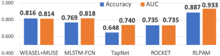
Figure 2: Performance Comparison on MIMIC-III dataset. ShapeNet cannot be implemented due to the high missing rate in clinical data which make shapelet based methods hard to converge.
proposed towards TS classification but can be directly applied to MTS classification. (iii) Three MTS classification benchmarks [Shokoohi-Yekta et al., 2015; Bagnall et al., 2018]: EDI is one nearest neighbor classifier based on Euclidean distance. DTWI is dimension-independent DTW. DTWD is dimension-dependent DTW.
4.4 Classification Results
The overall classification accuracy results for the UEA datasets are presented in Table 2. The result "N/A" indicates the corresponding methods are not reported in [Bagnall et al., 2018] or incapable of producing the results. Overall, RLPAM achieves the best average accuracy rank across all the compared methods. Specifically, RLPAM attains the average rank of 2.900, which is higher than all the baselines. RLPAM results in 14 wins/ties while the best performing state-of-theart gets 8 wins/ties. In terms of MPCE, RLPAM achieves the least average error per class across all datasets. In Friedman test, our statistical significance is p <= 0.001. It confirms the statistical significance of the performance difference among all 12 methods. The Wilcoxon signed-rank test is performed between RLPAM and all baselines, which shows that overall performance of RLPAM over the 30 UEA datasets outperforms baselines with statistical significance at the level of p < 0.05, except ROCKET and MiniRocket. Interestingly, on datasets where UCS performs reasonably well but not as good as the state-of-the-arts, RLPAM can improve its performance and even outperforms state-of-the-arts. On datasets where UCS performs poorly, RLPAM can significantly improve its performance but may not beat the state-of-the-arts. The observations above demonstrate the importance of generating pattern-based representations, as proposed in RLPAM, for MTS classification. Moreover, RLPAM performs better in most datasets that contain a limited number of training samples, such as StandWalkJump (SWJ) and AtrialFibrillation (AF) which contain only 12 and 15 training samples respectively. The reason could be that these datasets intrinsically contain high-qualitative representative and discriminative patterns which are captured by RLPAM.
We further investigate how RLPAM performs against the state-of-the-art MTS classification methods on a real-world healthcare problem, i.e., 24-hour early septic shock prediction. For this task we use the data extracted fromMIMIC-III, along with the open-sourced code attached to each method in its original paper. Given that this is a binary classification task, we show both the average accuracy and AUC obtained
| Classes | Pattern | Interpretation |
|---|---|---|
| Non-shock | N1 N2 N3 | Temperature Physiological Responses Inflammation, Slight Non-Temperature Inflammation Temperature Physiological Responses Inflammation Physiological Organ Failure, Slight Respiratory Organ Failure |
| Shock | S1 S2 S3 | Under-Resuscitated Septic Shock, Cardiovascular Organ Failure Under-Resuscitated Septic Shock, Respiratory Organ Failure, Cardiovascular Organ Failure Slight Under-Resuscitated Septic Shock, Slight Cardiovascular Organ Failure, Non-Temperature Physiological Response Inflammation |
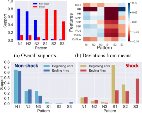
(c) Beginning/ending 4hrs' supports across two classes.
Figure 3: Analysis for the RLPAM informed patterns.
from 5-fold cross validation in Figure 2. It can be observed that RLPAM achieves the best performance in terms of both metrics, which significantly outperforms the other methods.
4.5 ACase Study on Interpretability
Six RLPAM patterns with the highest supports were selected here. Here the support is calculated by the portion of visits which contain the pattern among all visits. As shown in Figure 3a, three of them (i.e., N1, N2, N3) appear significantly more frequently in non-shock visits than in shock ones, while S1, S2, S3 appears significantly more in shock visits than non-shock ones. For each pattern l ∈ L and all MTS X = {X1, . . . ,XN}, we calculate the average value, κdl , of each attribute d ∈ [1, D] recorded in the part of X pertaining to Mi,l = 1, across all i ∈ [1,N] patients. In what follows, the deviations κdl - ¯κdl , from the population mean of each attribute ¯κdl = 1N ∑i 1 ti ∑t xi,t,d, are visualized in Figure 3b 2 . It can be observed that S1, S2, S3 in general result in negative deviations (shown in red), while most part of N1, N2, N3 are associated with positive deviations (shown in blue). According to the deviations, and referring to the septic shock diagnosis criteria provided by some expertized clinician, we find potential ways to interpret the patterns as shown in Table 3. The patterns informed by RLPAM are fine-grained and convey insights of septic shock progress.
2 All MTS X are min-max normalized before calculating deviations.
We further analyze the supports of patterns in the beginning 4 hours and the ending 4 hours across visits for non-shock and shock patients, which are shown in Figure 3c left and right side respectively. We find that patterns N1, N2, N3 appear consistently frequent across non-shock visits with similar supports between the beginning and the ending 4 hours. On the contrary, patterns S1, S2, S3 behave differently across shock visits: S1 is more than twice as frequent in the beginning 4 hours than in the ending 4 hours; S2 is consistently frequent in both the beginning and ending 4 hours; S3 only appears in the ending 4 hours. Interestingly, we also investigate all C = 6 cluster indices that constitute UCSs, and most of them have supports greater than 0.6 on both shock and non-shock classes. This indicates that it is hard to use cluster indices alone to differentiate classes, but the patterns recognized by RLPAM can provide insights into the relations between MTS and class labels.
5 Conclusion and Limitation
In this paper, we proposed a MTS classification framework called RLPAM. It first converted MTS into MPTS which contain information propagated from interpretable pattern candidates. Then, a deep RL module was devised to iteratively identify and refine the set of discriminative patterns in concurrent with training of a deep learning classifier. The design of the actor's neural architecture as well as the adapted actor-critic gradients updates were shown effective for maintaining the set of selected patterns in a sample-agnostic manner. We ran experiments on 30 UEA Archive datasets and the MIMIC-III dataset. The results showed that RLPAM outperforms state-of-the-art methods as well as the ablation baseline which directly using UCS as classification model inputs, illustrating the importance of identifying discriminative patterns. However, our performance was limited on datasets where UCS performs extremely poor; possibly due to the lack of graphical connectivity structure among temporal or crossattribute dependencies underlying the data, which makes the cluster indices generated by TICC not informative enough for downstream analyses. In the future, this could be resolved by designing event clustering method that could improve the expressiveness and representational power of its UCS outputs.
Acknowledgements
This research was supported by the NSF Grants: #2013502, #1726550, #1660878, #1651909, #1522107, #1837499, and #2112562, and by AFOSR FA9550-19-1-0169. Special thanks to John Hostetter (NCSU) for his insightful comments to help improve paper presentation.
@inproceedings{ijcai2022p415,
  title     = {A Reinforcement Learning-Informed Pattern Mining Framework for Multivariate Time Series Classification},
  author    = {Gao, Ge and Gao, Qitong and Yang, Xi and Pajic, Miroslav and Chi, Min},
  booktitle = {Proceedings of the Thirty-First International Joint Conference on
               Artificial Intelligence, {IJCAI-22}},
  publisher = {International Joint Conferences on Artificial Intelligence Organization},
  editor    = {Luc De Raedt},
  pages     = {2994--3000},
  year      = {2022},
  month     = {7},
  note      = {Main Track},
  doi       = {10.24963/ijcai.2022/415},
  url       = {https://doi.org/10.24963/ijcai.2022/415},
}
TY - CPAPER TI - A Reinforcement Learning-Informed Pattern Mining Framework for Multivariate Time Series Classification AU - Gao, Ge AU - Gao, Qitong AU - Yang, Xi AU - Pajic, Miroslav AU - Chi, Min T2 - Proceedings of the Thirty-First International Joint Conference on Artificial Intelligence, IJCAI-22 PB - International Joint Conferences on Artificial Intelligence Organization PY - 2022 SP - 2994 EP - 3000 DO - 10.24963/ijcai.2022/415 UR - https://doi.org/10.24963/ijcai.2022/415 ER -Copied
Machine-readable versions of this paper, for tools and AI agents:





