
Learning Continuous Graph Structure with Bilevel Programming for Graph Neural Networks
Proceedings of the Thirty-First International Joint Conference on Artificial Intelligence. Main Track. Pages 3057-3063.
https://doi.org/10.24963/ijcai.2022/424
Keywords
- Computer Vision: Scene analysis and understanding
- Machine Learning: Hyperparameter Optimization
- Data Mining: Mining Graphs
Abstract
Learning graph structure for graph neural networks (GNNs) is crucial to facilitate the GNN-based downstream learning tasks. It is challenging due to the non-differentiable discrete graph structure and lack of ground-truth. In this paper, we address these problems and propose a novel graph structure learning framework for GNNs. Firstly, we directly model the continuous graph structure with dual-normalization, which implicitly imposes sparse constraint and reduces the influence of noisy edges. Secondly, we formulate the whole training process as a bilevel programming problem, where the inner objective is to optimize the GNNs given learned graphs, while the outer objective is to optimize the graph structure to minimize the generalization error of downstream task. Moreover, for bilevel optimization, we propose an improved Neumann-IFT algorithm to obtain an approximate solution, which is more stable and accurate than existing optimization methods. Besides, it makes the bilevel optimization process memory-efficient and scalable to large graphs. Experiments on node classification and scene graph generation show that our method can outperform related methods, especially with noisy graphs.
- [Bengio et al., 2013] Y. Bengio, N. Léonard, and A. Courville. Es- timating or propagating gradients through stochastic neurons for conditional computation. arXiv:1308.3432, 2013.
- [Chen et al., 2020] Y. Chen, L. Wu, and M. Zaki. Iterative deep graph learning for graph neural networks: Better and robust node embeddings. In NeurIPS, 2020.
- [Colson et al., 2007] B. Colson, P. Marcotte, and G. Savard. An overview of bilevel optimization. Annals of Operations Research, 2007.
- [Fatemi et al., 2021] B. Fatemi, L. El Asri, and S.M. Kazemi. Slaps: Self-supervision improves structure learning for graph neural networks. In NeurIPS, 2021.
- [Franceschi et al., 2019] L. Franceschi, M. Niepert, M. Pontil, and X. He. Learning discrete structures for graph neural networks. In ICML, 2019.
- [Franklin, 2012] J.N. Franklin. Matrix theory. Courier Corporation, 2012.
- [Gao and Ji, 2019] H. Gao and S. Ji. Graph u-nets. In ICML, 2019.
- [Ghadimi and Wang, 2018] S. Ghadimi and M. Wang. Approxima- tion methods for bilevel programming. arXiv:1802.02246, 2018.
- [Golub and Loan, 2013] G.H. Golub and C.F. Van Loan. Matrix computations. JHU press, 2013.
- [Grazzi et al., 2020] R. Grazzi, L. Franceschi, M. Pontil, and S. Salzo. On the iteration complexity of hypergradient compu- tation. In ICML, 2020.
- [Hamilton et al., 2017] W. Hamilton, Z. Ying, and J. Leskovec. In- ductive representation learning on large graphs. In NeurIPS, 2017.
- [He et al., 2020] X. He, K. Deng, X. Wang, Y. Li, Y. Zhang, and M. Wang. Lightgcn: Simplifying and powering graph convolu- tion network for recommendation. In SIGIR, 2020.
- [Henaff et al., 2015] M. Henaff, J. Bruna, and Y. LeCun. Deep con- volutional networks on graph-structured data. arXiv:1506.05163, 2015.
- [Huang and Carley, 2019] B. Huang and K. Carley. Syntax-aware aspect level sentiment classification with graph attention net- works. In EMNLP, 2019.
- [Jang et al., 2017] E. Jang, S. Gu, and B. Poole. Categorical repa- rameterization with gumbel-softmax. In ICLR, 2017.
- [Jiang et al., 2019] B. Jiang, Z. Zhang, D. Lin, J. Tang, and B. Luo. Semi-supervised learning with graph learning-convolutional net- works. In CVPR, 2019.
- [Jin et al., 2020] W. Jin, Y. Ma, X. Liu, X. Tang, S. Wang, and J. Tang. Graph structure learning for robust graph neural net- works. In SIGKDD, 2020.
- [Kazi et al., 2020] A. Kazi, L. Cosmo, N. Navab, and M. Bronstein. Differentiable graph module (dgm) for graph convolutional net- works. arXiv:2002.04999, 2020.
- [Kingma and Welling, 2013] D.P. Kingma and M. Welling. Auto- encoding variational bayes. arXiv:1312.6114, 2013.
- [Kipf and Welling, 2017] T.N. Kipf and M. Welling. Semi- supervised classification with graph convolutional networks. In ICLR, 2017.
- [Kool et al., 2019] W. Kool, H. Van Hoof, and M. Welling. Stochas- tic beams and where to find them: The gumbel-top-k trick for sampling sequences without replacement. In ICML, 2019.
- [Li et al., 2016] Y. Li, D. Tarlow, M. Brockschmidt, and R. Zemel. Gated graph sequence neural networks. In ICLR, 2016.
- [Li et al., 2021] R. Li, S. Zhang, B. Wan, and X. He. Bipartite graph network with adaptive message passing for unbiased scene graph generation. In CVPR, 2021.
- [Lorraine et al., 2020] J. Lorraine, P. Vicol, and D. Duvenaud. Op- timizing millions of hyperparameters by implicit differentiation. In AISTATS, 2020.
- [Pearlmutter, 1994] B.A. Pearlmutter. Fast exact multiplication by the Hessian. Neural Computation, 1994.
- [Qu et al., 2020] M. Qu, T. Gao, L. Xhonneux, and J. Tang. Few- shot relation extraction via bayesian meta-learning on relation graphs. In ICML, 2020.
- [Rudin, 1964] W. Rudin. Principles of mathematical analysis. McGraw-hill New York, 1964.
- [Veličković et al., 2018] P. Veličković, G. Cucurull, A. Casanova, A. Romero, P. Liò, and Y. Bengio. Graph attention networks. In ICLR, 2018.
- [Wan and Kokel, 2021] G. Wan and H. Kokel. Graph sparsification via meta-learning. DLG@AAAI, 2021.
- [Wang et al., 2020] X. Wang, M. Zhu, D. Bo, P. Cui, C. Shi, and J. Pei. Am-gcn: Adaptive multi-channel graph convolutional net- works. In SIGKDD, 2020.
- [Wu et al., 2018] Z. Wu, B. Ramsundar, E.N. Feinberg, J. Gomes, C. Geniesse, A.S. Pappu, K. Leswing, and V. Pande. Molecu- lenet: a benchmark for molecular machine learning. Chemical science, 2018.
- [Wu et al., 2019] H. Wu, C. Wang, Y. Tyshetskiy, A. Docherty, K. Lu, and L. Zhu. Adversarial examples on graph data: Deep insights into attack and defense. In IJCAI, 2019.
- [Xu et al., 2017] D. Xu, Y. Zhu, C.B. Choy, and L. Fei-Fei. Scene graph generation by iterative message passing. In CVPR, 2017.
- [Xu et al., 2018] K. Xu, C. Li, Y. Tian, T. Sonobe, K. Kawarabayashi, and S. Jegelka. Representation learning on graphs with jumping knowledge networks. In ICML, 2018.
- [Xu et al., 2019] B. Xu, H. Shen, Q. Cao, Y. Qiu, and X. Cheng. Graph wavelet neural network. In ICLR, 2019.
- [Yu et al., 2020] F. Yu, Y. Zhu, Q. Liu, S. Wu, L. Wang, and T. Tan. Tagnn: Target attentive graph neural networks for session-based recommendation. In SIGIR, 2020.
- [Zhang and Zitnik, 2020] X. Zhang and M. Zitnik. Gnnguard: De- fending graph neural networks against adversarial attacks. In NeurIPS, 2020.
- [Zheng et al., 2020] C. Zheng, B. Zong, W. Cheng, D. Song, J. Ni, W. Yu, H. Chen, and W. Wang. Robust graph representation learning via neural sparsification. In ICML, 2020.
- [Zügner and Günnemann, 2019] D. Zügner and S. Günnemann. Adversarial attacks on graph neural networks via meta learning. In ICLR, 2019.
References were extracted automatically from the PDF and may contain errors.
Full text extracted automatically from the PDF; figures, tables and equations may differ. The PDF is the version of record.
1 Introduction
Graphs have been widely used in various domains, such as social networks, biology and chemistry, where data are non-Euclidean and has complex relationships. Recently, graph neural networks (GNNs) [Veliˇckovi´c et al., 2018; Kipf and Welling, 2017; Li et al., 2016; Xu et al., 2018; Xu et al., 2019] have extended the advantages of deep neural networks to graphs and brought significant performance improvement on many real-world problems, including computer vision [Xu et al., 2017; Li et al., 2021], natural language processing [Henaff et al., 2015; Huang and Carley, 2019; Qu et al., 2020], recommendation [Yu et al., 2020; He et al., 2020], biology [Wu et al., 2018; Gao and Ji, 2019], and so on.
For various real-world problems, constructing reasonable graphs from data is crucial to guarantee the effectiveness of GNNs. However, the graphs naturally constructed from domain data are often noisy or incomplete, thus not optimal for the downstream tasks. Instead, a more promising solution is to learn the graph structure to facilitate the subsequent learning process based on GNNs. There are two main challenges in graph structure learning: Firstly, optimizing a discrete graph structure is a non-differentiable problem, so the commonly used back-propagation with gradient descent cannot apply. Secondly, most real-world learning tasks provide no supervision information of underlying graph structures, i.e., the ground-truth graph structure is usually unknown.
To overcome the non-differentiable problem, many works relax the binary graph structure as a real-valued weighted adjacency matrix A ∈ [0, 1]N×N and use extra post-processing operation to prune edges according to edge weights [Jiang et al., 2019; Wang et al., 2020; Chen et al., 2020; Zhang and Zitnik, 2020]. With this continuous relaxation, the output of GNNs can be differentiable with respect to the graph structure. An alternative approach is to model the edge probability over graphs, and sample from the edge probability distribution to acquire discrete graph structure [Franceschi et al., 2019; Zheng et al., 2020; Kazi et al., 2020]. The main obstacle to this solution is how to make the sampling operation differentiable and enable optimization with gradient descent methods. Inspired by variational approaches [Kingma and Welling, 2013], several recent studies [Franceschi et al., 2019; Zheng et al., 2020; Kazi et al., 2020] are able to make the sampling process differentiable by adopting reparameterization tricks, like straight-through estimator [Bengio et al., 2013], Gumbel-Softmax [Jang et al., 2017] and Gumbel-Topk trick [Kool et al., 2019]. Although the continuous relaxation and probabilistic sampling approaches have achieved encouraging results, these methods still have some limitations. The continuous relaxation methods are usually sensitive to the hyper-parameters in the post-processing operation, especially at the presence of noisy edges. Most probabilistic sampling methods have poor convergence speed and require extra inference time due to the sampling operation.
To address the lack of supervision information problem, some research works have been proposed recently. A direct solution is simultaneously optimizing the graph structure and GNN parameters with the training loss of downstream task, which is easy to cause over-fitting or edge starvation [Fatemi et al., 2021]. A better way is to use prior knowledge as supervision to optimize the graph structure. Some methods [Jin et al., 2020; Chen et al., 2020; Wang et al., 2020] construct the graph regularization loss by utilizing some assumptions of graph property, like feature smoothness, graph sparsity and low-rank. Other methods [Fatemi et al., 2021] introduce auxiliary self-supervised tasks to incorporate the prior knowledge for graph structure learning. Although these methods can generate good graphs for some specific tasks, the generalization ability is limited as the prior knowledge is usually task-specific and only suitable for known datasets.
In this work, we propose a novel continuous graph structure learning framework, namely Learning Continuous Graph Structure (LCGS), to address both problems. Firstly, we construct normalized graph structure, whose elements are naturally continuous and range from 0 to 1. Then, we propose dual-normalization to renormalize the continuous graph structure and implicitly impose sparse constraint, thus significantly reduce the influence of noisy edges. Secondly, we formulate graph structure learning and GNN parameters learning as a bilevel programming problem, where the inner objective is to optimize the GNN given the learned graph for a specific task, while the outer objective is to optimize the graph structure to minimize the generalization error. In this way, the inter-dependency between graph structure learning and GNN parameters learning is fully exploited. The target of the downstream task acts as the indirect supervisory information for the graph structure learning.
For bilevel optimization, existing studies [Franceschi et al., 2019; Wan and Kokel, 2021] usually unroll the inner optimization dynamics every T steps, then calculate the hypergradient (outer level gradient) through the unrolled dynamics. However, the unrolled differentiation methods require high-order derivatives, which incur non-trivial memory and computational cost, especially as the number of unrolled dynamics T increases. In this paper, instead of unrolling the inner optimization, we derive an analytical expression for the hypergradient computation based on Neumann-IFT algorithm [Lorraine et al., 2020; Grazzi et al., 2020], in which the hypergradient depends only on the solution instead of the path of the inner optimization. Moreover, based on the theoretical analysis on the convergence condition of Neumann series theorem, we propose improved Neumann-IFT algorithm which makes the Neumann approximation more stable and closer to the true inverse Hessian. Besides, the improved NeumannIFT algorithm does not store nor differentiate through the inner optimization path, which makes the bilevel optimization process memory-efficient and scalable to large graphs.
In summary, our main contributions are as follows:
- We propose dual-normalization on continuous graph structures, which implicitly imposes sparse constraint and significantly reduces the influence of noisy edges.
- We formulate continuous graph structure learning and GNN parameters learning as a bilevel programming problem, where the generalization error on downstream tasks supervises the learning of graph structures.
- We propose improved Neumann-IFT algorithm to solve the bilevel optimization problem, which is not only more
- stable and accurate than the original approximation algorithm, but also memory-efficient and scalable.
- We conduct a series of experiments and ablation studies on node classification and scene graph generation tasks, which shows that our method can outperform related methods in various situations.
2 Background
We first introduce some background about graph neural networks and bilevel programming.
2.1 Graph Neural Networks
Let G = (V, E) be a graph, where V = {vi}Ni=1 is the vertex set and E ⊆ V ×V is the edge set. We denote the node feature matrix as X ∈ RN×F , where xi ∈ RF is the feature of node vi. An adjacency matrix A can describe the connections between N vertices: Aij = 1 if there is an edge between vi and vj, and Aij = 0 otherwise. The degree matrix D is a diagonal matrix with Dii = ΣjAij and Dij = 0 if i ̸= j.
Based on graph G, many learning tasks can be solved using GNNs. For example, given the adjacency matrix A, the node feature matrix X and the vector of node labels Y , the goal of node classification is to learn a function fw that maps the nodes to their predicted class labels ˆ Y = fw(X,A) by minimizing the regularized empirical loss:
where w is the parameter vector of fw, l is a loss function to measure the summarized difference between the predicted and true labels, and Ω is a regularization function. As an example of function fw, a graph convolutional network (GCN) with two hidden layers is proposed by [Kipf and Welling, 2017] for undirected graph, which is expressed as
where w = (W1, W2) are the parameters of the GCN and ˆ A is the normalized adjacency matrix, ˆ A = ˜D-1/2 (A+ I) ˜D-1/2 with ˜D =D+ I.
2.2 Bilevel Programming
Bilevel programs are optimization problems where a set of variables occurring in one objective function are constrained to be an optimal solution of another objective function. Formally, given two objective functions F and L, and two sets of variables, θ ∈ Rm and w ∈ Rd , a bilevel program is given by
where F and L are called outer and inner objectives, θ and w are called outer and inner variables, respectively.
3 Learning Continuous Graph Structure
In this work, we propose a novel continuous graph structure learning framework, LCGS. In Section 3.1, we will introduce how to model the normalized graph structure and how to to impose sparse constraint with dual-normalization. In Section 3.2, we will explain the formulation of the bilevel problem, and how to optimize the graph structure learning parameters by minimizing the generalization error. Then, we will introduce the improved Neumann-IFT, a better optimization algorithm for the bilevel program in Section 3.3. Finally, we will compare our method with related works in Section 3.4.
3.1 Constructing Continuous Graph with Dual-normalization for GNNs
Graph structure learning is a non-differentiable optimization problem, due to the discrete graph structure. To address this limitation, in this paper, we try to learn the normalized graph structure, whose elements are close to be continuous. To this end, we train a graph generator parameterized by θ ∈ Rm to generate the normalized graph structure O = (oij)N×N given the node feature X and the prior adjacency matrix (may not exist). As an example, we can use the symmetric normalized graph ˆ A as initialized O, for semi-supervised node classification task with GCN. In this case, θ = vec(O) and m = N ×N.
However, after several optimization steps, it is possible that O becomes a dense matrix and ∑i oui ≫ ∑i ovi for node u and v, which will introduce much noise and cause optimization difficulties. To address these problems, we try to constrain O and renormalize it as:
where g(·) is a renormalization function. For node classification, we use the symmetric normalization function as
where c is a non-negative integer. When c ≥ 1, we can use c to compensate renormalized ˆ oii and control the sparsity of ˆO. With a large c, the non-diagonal elements of ˆO will decrease, which makes ˆO sparse. When c →∞, ˆO is sparse enough to be an identity matrix. In practice, we find that a proper c can significantly reduce the influence of noisy edges.
Considering the initialization with normalized graph and renormalization operation, we call the graph construction method as dual-normalization. With dual-normalization, the GCN formulation can be expressed as
With a slight modification, the dual-normalization method can also be used in inductive learning tasks with different GNN backbones. See the method instantiation for scene graph generation in Appendix D 1 .
3.2 Jointly Learning Graph Structure and GNNs
Now, we have two sets of learnable parameters θ ∈ Rm and w ∈ Rd , which are involved in learning graph structure and GNN parameters, separately. The problem is how to define the objective functions of the two learning tasks. As some previous work [Franceschi et al., 2019] points out that the graph structure learning and GNN parameter learning are closely dependent. On the one hand, the optimal w can be obtained by minimizing the loss of the downstream task given the underlying graph structure parameterized by θ, i.e., wθ = argminw L(w, θ). On the other hand, θ should be optimized to maximize the generalization ability of GNNs for test cases.
1 See appendix in https://github.com/hu-my/LCGS-appendix.
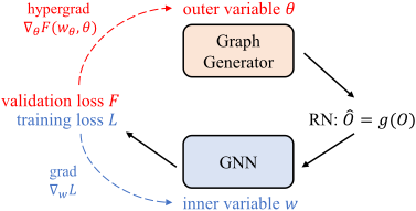
In this case, we use a subset of training instances, (Xval, Yval) (the Validation set), from which we can estimate the generalization error. Hence, a graph generator parameterized by θ can be learned by minimizing the following objective:
Joint optimizing the two objectives L and F can be formulated as a bilevel programming problem [Colson et al., 2007]:
The outer objective F aims to find the optimal continuous dual-normalized graph structure and the inner objective L aims to find the optimal parameters of GNNs given the graph. A sketch of LCGS framework is presented in Fig. 1 and the overall algorithm can be seen in Appendix B.
3.3 Hypergradient Computation by Improved Neumann-IFT
Now we discuss how to solve the bilevel programming problem defined in Eq. (8). For the inner objective, we can use stochastic gradient descent (SGD) to optimize the inner variables w:
where αt is a learning rate. For the outer objective, a hypergradient descent is performed to update graph generator as:
where βt is the outer learning rate. Assuming that, after T iterations, wθ,T is the minimizer of the loss function L with fixed graph generator parameter θ, we can use it to calculate the hypergradient ∇θF as
Algorithm 1 Improved Neumann-IFT
Input: L(w, θ), F(w, θ).
Parameter: K, S.
- 1: ˆλn ←Power Iteration(wθ,t, ∂wL(wθ,t, θ), S)
- 2: γ ← 1 ˆλn
- 3: Initialize v, p ← ∂wF(wθ,t, θ)
- 4: for j = 1 →K do
- 5: v ← v -γ ∗ vector-Hessian(v, ∂ 2w,w L(wθ,t, θ))
- 6: p ← p+ v
- 7: end for
- 8: g ←vector-Jacobian(γ ∗ p, ∂ 2w,θ L(wθ,t, θ))
- 9: return ∂θF(wθ,t, θ) - g {Approximate hypergradient}
Hypergradient Computation
The hypergradient computation in Eq. (11) consists of two parts: direct gradient (the first item) and indirect gradient (the second item). The indirect gradient is difficult to compute, especially for the parameter Jacobian ∂w ∂θ , because we must account for how the optimal parameters w change with respect to θ. Inspired by Neumann-IFT algorithm [Lorraine et al., 2020], we can approximately estimate the Jacobian based on implicit function theorem [Rudin, 1964] and Neumann series theorem [Franklin, 2012].
If there exists one point (w′ , θ′ ) with ∂L(w,θ) ∂w |(w′ ,θ′ ) = 0, through implicit function theorem, we can replace parameter Jacobian ∂w ∂θ with product of inverse Hessian matrix and mixed partial derivative:
Then, Neumann-IFT uses Neumann series theorem to estimate inverse Hessian as:
For computation efficiency, only the first K terms of Neumann series are usually used as approximation. Thus, the final hypergradient is approximately computed as:
Improved Neumann-IFT Algorithm
There is an important issue with the above approximate computation: using the Neumann series theorem to estimate the inverse Hessian must subject to the condition that I-γ∗ ∂ 2L ∂w∂w is a convergent matrix, which is not guaranteed in above computation. In this paper, we improve Neumann-IFT to address this issue and give an efficient method to meet the condition.
Firstly, we derive how to make I - γ ∗ ∂ 2L ∂w∂w a convergent matrix by scaling the constant γ. Suppose A is a square matrix with n eigenvalues {λi}ni=1 , ρ(A) = maxi |λi| is the spectral radius of A. It is well-known that A is a convergent matrix if and only if ρ(A) < 1 [Golub and Loan, 2013]. Then, the problembecomes how tomake ρ(I-γ∗ ∂ 2L ∂w∂w ) < 1 by scaling γ.
Theorem 1 (Matrix Convergence Condition). Suppose A is a positive definite matrix with n eigenvalues 0 < λ1 ≤ . . . ≤ λn, where λn is the maximum eigenvalue, I - γA is a convergent matrix if γ ∈ (0, 2 λn ).
Since theHessianmatrix ∂ 2L ∂w∂w is a symmetric positive definite matrix, we can set γ to a small enough value to make I -γ ∗ ∂ 2L ∂w∂w a convergent matrix. However, it is not the case that the smaller γ the better.
Theorem 2 (Approximation Error Upper Bound). Suppose ∂ 2L ∂w∂w is a positive definite matrix and I - γ ∗ ∂ 2L ∂w∂w is a convergent matrix, if we use the first K terms of Neumann series to estimate (γ ∗ ∂ 2L ∂w∂w )-1 , the approximation error is upper bounded by ∥I-γ∗ ∂2 L ∂w∂w ∥K+1 2 1-∥I-γ∗ ∂2L ∂w∂w ∥2 . When γ ∈ (0, 2 λ1+λn ), with the increase of γ, the upper bound decreases.
From Theorem 2, we find that with a smaller γ, we need more Neumann terms to get an accurate hypergradient. On the contrary, with a larger γ, we can use shorter Neumann series to estimate hypergradient with less computation. So, it is vital to set γ close to the bound 2 λ1+λn .
Next, we propose an efficient way to estimate the maximum eigenvalue λn and set the value of γ. Due to the large size of the Hessian matrix ∂ 2L ∂w∂w , it is infeasible to explicitly save and factorize it to compute the maximum eigenvalue. In this case, we adopt Power Iteration method [Golub and Loan, 2013] with vector-Hessian product [Pearlmutter, 1994] to estimate the dominate eigenvalue ˆλn (equivalent to the maximum eigenvalue in this case). Then, we can set γ = 1 ˆλn , which can meet the condition of γ ≤ 2 λ1+λn .
We outline the improved Neumann-IFT algorithm in Algorithm 1. Note that we use Power Iteration to estimate ˆλn at line 1, which involves S times vector-Hessian products. At lines 4-7, we also use vector-Hessian products to calculate the sum of first K terms of Neumann series.
3.4 Comparisons to RelatedWorks
The LCGS framework and improved Neumann-IFT algorithm described in Section 3.1 and 3.3 address several issues that have been studied by some previous approaches in graph structure learning and bilevel optimization:
- Some previous methods [Wang et al., 2020; Chen et al., 2020; Zhang and Zitnik, 2020] try to address the non-differentiation problem by representing the discrete graph structure as a weighted adjacency matrix, then
use post-processing operations to make the weighted adjacency matrix sparse. However, they are sensitive to the choice of hyper-parameters and a suitable similarity measure. In this paper, we directly model the normalized graph structure and introduce dual-normalization to implicitly impose the sparse constraint, without explicit post-processing operations to prune edges.
- Computationally, improved Neumann-IFT is more efficient in solving bilevel program than unrolled differentiation. For any vector v ∈ Rd , let O(n1) and O(n2) denote the space complexities for product v ∗ ∂ 2w,w L and v ∗ ∂ 2w,θ L, respectively. Unrolled differentiation method needs O(T(n1 + n2) + Td) space [Franceschi et al., 2019], while improved Neumann-IFT only needs O((K + S)n1 + n2), where O(Sn1) is the space complexity for estimating the maximum eigenvalue by Power Iteration. For large graphs with O(n2) ≫ O(n1), the space complexity of improved Neumann-IFT will be much less than unrolled differentiation.
- Assume the inner objective L has Lg-Lipschitz continuous gradient condition and µg-strongly convexity, previous work [Ghadimi and Wang, 2018] has proved the approximation error upper bound as 1 µg (1 - µg Lg )K+1 . With the same assumption, our bound is tighter than it when γ = 1 Lg . Moreover, we explore the range of γ and how to set an appropriate γ to reduce the approximation error bound from the view of computation.
4 Experiments
We perform comprehensive experiments on the semisupervised node classification task, which is a transductive learning task and usually used for evaluating the GNN performance. We also report results on inductive Scene Graph Generation (SGG) task to show the applicability of our method. Due to the page limit, we will show the results of node classification in the next subsections and show the results of SGG task in Appendix D.
4.1 Settings
Datasets. We conduct experiments on three citation network datasets (Cora, Citeseer, Pubmed). The nodes in a citation network represent documents and edges correspond to citation link. Node features are the sparse bag-of-words representations of the documents and node labels indicate the topic class of the documents.
Tasks and Setup. To evaluate our method, we apply LCGS to semi-supervised node classification in two scenarios: (1) the underlying graph is normal; (2) the underlying graph is noisy. For the normal graph scenario, we use the same dataset split and experimental setup as previous work [Kipf and Welling, 2017]. For the noisy graph scenario, we perturb the graph by the non-targeted attack method, which is usually used in graph adversarial attack domain. In our experiments, we adopt a representative non-targeted attack method, metattack [Z¨ugner and G¨unnemann, 2019], to perturb graphs by adding or removing edges. Following [Z¨ugner and G¨unnemann, 2019; Jin et al., 2020], we use 10% labeled data for training, the rest 10% labeled data for validation and 80% unlabeled data for test. In all experiments, we run 10 times with different random seed then report the average results with standard deviation. See more details about dataset statistics and implementation details in Appendix C.
| Cora | Citeseer | Pubmed | |
|---|---|---|---|
| GCN | 81.5 (-) | 70.3 (-) | 79.0 (-) |
| GAT | 83.0 (0.7) | 72.5 (0.7) | 79.0 (0.3) |
| GraphSAGE | 77.4 (1.0) | 67.0 (1.0) | 76.6 (0.8) |
| GCN-Jaccard | 78.8 (0.5) | 71.7 (0.4) | 79.2 (0.3) |
| Pro-GNN | 81.2 (0.4) | 71.9 (0.4) | - |
| LDS | 84.1 (0.4) | 75.0 (0.4) | - |
| IDGL | 84.5 (0.3) | 74.1 (0.2) | - |
| IDGL-ANCH | 84.4 (0.2) | 72.0 (1.0) | 83.2 (0.2) |
| LCGS | 85.0 (0.4) | 75.9 (0.2) | 82.3 (0.3) |
ComparativeMethods. We compare our method with several previous graph structure learning methods: (1) GCNJaccard [Wu et al., 2019], (2) Pro-GNN [Jin et al., 2020], (3) LDS [Franceschi et al., 2019], (4) IDGL and a variant IDGLANCH [Chen et al., 2020]. Furthermore, we include many GNN variants (i.e., vanilla GCN [Kipf and Welling, 2017], GAT [Veliˇckovi´c et al., 2018] and GraphSAGE [Hamilton et al., 2017]) as baselines, which are based on fixed graph.
4.2 Experimental Results
Table 1 shows the results on normal graphs. First of all, compared to other methods, our model achieves best results on two of three datasets. Besides, unlike some methods (ProGNN, LDS and IDGL) which cannot handle large graphs, e.g., Pubmed dataset, LCGS still works effectively. This benefits from the memory-efficient optimization algorithm and implicit sparse constraint by dual-normalization.
Table 2 shows the results against noisy graphs. Compared to GCN and GAT, LCGS achieves better or comparable results in different perturbation intensities, which shows learning underlying graph structure do improve GNN performance. Moreover, in comparison with other graph structure learning methods, LCGS provides competitive results on Cora and Citeseer when the perturbation rate is small and significantly outperforms others with larger perturbation rate. This verifies that our LCGS has stronger robustness thus performs better in noisy environment.
4.3 Ablation Study
In this subsection, we do some ablation studies to explore the influence of each component in LCGS and effectiveness of improved Neumann-IFT algorithm for approximate solution.
Influence of Each Component
The core of our method is the dual-normalization and improved Neumann-IFT algorithm. To verify their effectiveness, we remove either the dual-normalization or improved Neumann-IFT. For the former, we replace Eq. (6) with the original GCN formulation Eq. (2); for the latter, we use the Neumann-IFT with a fixed γ instead of improved NeumannIFT algorithm. In Table 3, we compare three options: (A) LCGS without dual-normalization and improved NeumannIFT; (B) LCGS without dual-normalization; (C) LCGS without improved Neumann-IFT. We conduct experiments on both normal and noisy graph scenarios. For simplicity, we only set the Ptb Rate = 0.25 for the noisy graph scenario.
| Dataset | Ptb Rate (%) | GCN | GAT | GCN-Jaccard | Pro-GNN | LDS | IDGL | Ours |
|---|---|---|---|---|---|---|---|---|
| Cora | 0 | 83.5 (0.4) | 84.0 (0.7) | 82.1 (0.5) | 83.0 (0.2) | 85.1 (0.4) | 85.3 (0.2) | 84.8 (0.3) |
| 5 | 76.6 (0.8) | 80.4 (0.7) | 79.1 (0.6) | 82.3 (0.5) | 81.6 (0.8) | 80.7 (0.2) | 81.2 (0.8) | |
| 10 | 70.4 (1.3) | 75.6 (0.6) | 75.2 (0.8) | 79.0 (0.6) | 79.2 (0.8) | 79.0 (0.3) | 79.8 (0.4) | |
| 15 | 65.1 (0.7) | 69.8 (1.3) | 78.2 (0.8) | 76.7 (0.5) | 71.0 (0.6) | 76.4 (1.3) | 78.6 (0.3) | |
| 20 | 59.6 (2.7) | 59.9 (0.9) | 65.7 (0.9) | 73.3 (1.6) | 75.3 (1.2) | 76.0 (0.8) | 76.9 (0.3) | |
| 25 | 47.5 (2.0) | 54.8 (0.7) | 60.8 (1.1) | 69.7 (1.7) | 72.2 (0.6) | 73.8 (0.4) | 75.5 (0.7) | |
| Citeseer | 0 | 72.0 (0.6) | 73.3 (0.8) | 72.1 (0.6) | 73.3 (0.7) | 75.7 (0.6) | 74.5 (0.5) | 75.8 (0.2) |
| 5 | 70.9 (0.6) | 72.9 (0.8) | 70.5 (1.0) | 72.9 (0.6) | 73.7 (0.3) | 71.9 (0.3) | 75.6 (0.3) | |
| 10 | 67.6 (0.9) | 70.6 (0.5) | 69.5 (0.6) | 72.5 (0.8) | 71.9 (0.6) | 69.2 (1.7) | 74.6 (0.2) | |
| 15 | 64.5 (1.1) | 69.0 (1.1) | 66.0 (0.9) | 72.0 (1.1) | 70.6 (0.8) | 67.5 (2.8) | 74.9 (0.4) | |
| 20 | 62.0 (3.5) | 61.0 (1.5) | 59.3 (1.4) | 70.0 (2.3) | 68.1 (0.4) | 67.0 (1.8) | 73.5 (0.5) | |
| 25 | 56.9 (2.1) | 61.9 (1.1) | 59.9 (1.5) | 69.0 (2.8) | 69.4 (0.8) | 69.7 (1.1) | 74.9 (0.3) |
| GCN | LCGS-A | LCGS-B | LCGS-C | LCGS | |
|---|---|---|---|---|---|
| Cora | 81.5 (-) | 83.5 (0.2) | 83.5 (0.2) | 84.6 (0.3) | 85.0 (0.4) |
| Citeseer | 70.3 (-) | 74.2 (0.5) | 75.1 (0.5) | 76.0 (0.3) | 75.9 (0.2) |
| Cora | 47.5 (2.0) | 54.7 (0.6) | 56.0 (0.7) | 75.2 (0.3) | 75.5 (0.7) |
| Citeseer | 56.9 (2.1) | 61.3 (0.5) | 64.8 (1.0) | 74.4 (0.2) | 74.9 (0.3) |
Table 3 shows that B is better than A on both normal and noisy graph scenarios, which show the improved NeumannIFT can enhance the graph generation capability and hypergradient estimation. C is marginally better than A and B on the normal graph scenario, while significantly outperforms them on the noisy graph scenario. This comparison shows that dual-normalization improves the robustness of model. We attribute this to the implicit sparse constraint introduced by dual-normalization. Moreover, with improved NeumannIFT and dual-normalization, LCGS can get comparative or better performances than both B and C.
Exploration for Improved Neumann-IFT
To further explore the effectiveness of improved NeumannIFT, based on the option C, we set γ in Neumann-IFT algorithm to different fixed values. The experimental results are presented in Table 4. First of all, we can find that, with the increase of γ, the performance tends to increase at first then decrease. This phenomenon is consistent with our theoretic analysis on the convergence condition and the upper bound of approximation error. Secondly, LCGS with improved Neumann-IFT is competitive to the best-compared baseline, without a heavy computational overhead. Note that when γ = 40, Neumann-IFT can have a slightly better result than the improved Neumann-IFT. We argue this is because the estimated maximum eigenvalue by Power Iteration method is not accurate enough. However, with the Power Iteration, we can get a proper γ adaptively and automatically, without trialand-errors per dataset and per hyper-parameters combination.
| Cora | Citeseer | |||
|---|---|---|---|---|
| Accuracy | Time | Accuracy | Time | |
| γ = 5 | 84.5 (0.3) | 9.4 (0.2) | 74.9 (0.4) | 14.6 (0.4) |
| γ = 10 | 84.7 (0.3) | 9.5 (0.2) | 75.5 (0.2) | 15.5 (0.4) |
| γ = 20 | 84.6 (0.3) | 10.0 (0.4) | 75.8 (0.2) | 15.6 (0.6) |
| γ = 40 | 81.6 (1.4) | 10.3 (0.3) | 76.0 (0.3) | 15.3 (0.7) |
| γ = 60 | 78.7 (1.9) | 9.3 (0.4) | 67.1 (5.5) | 14.8 (0.4) |
| LCGS | 85.0 (0.4) | 10.6 (0.3) | 75.9 (0.2) | 16.3 (0.6) |
5 Conclusion
This paper studies graph structure learning problem, which aims to find an optimal graph structure to facilitate the downstream task. To address the non-differentiation problem, we model the continuous graph structure with dualnormalization, which implicitly imposes the sparse constraint. Considering the inter-dependency between graph structure learning and GNN parameters learning, we formulate the whole learning process as a bilevel programming problem. For bilevel optimization, we propose an improved Neumann-IFT algorithm, which makes the approximation more stable and achieves better performance. Experiments show our method can achieve state-of-the-art performance on node classification and scene graph generation, which demonstrates the effectiveness of our LCGS framework.
Acknowledgments
This work is partially supported by Natural Science Foundation of China (NSFC): 61976203, 61876171 and U19B2036.
@inproceedings{ijcai2022p424,
  title     = {Learning Continuous Graph Structure with Bilevel Programming for Graph Neural Networks},
  author    = {Hu, Minyang and Chang, Hong and Ma, Bingpeng and Shan, Shiguang},
  booktitle = {Proceedings of the Thirty-First International Joint Conference on
               Artificial Intelligence, {IJCAI-22}},
  publisher = {International Joint Conferences on Artificial Intelligence Organization},
  editor    = {Luc De Raedt},
  pages     = {3057--3063},
  year      = {2022},
  month     = {7},
  note      = {Main Track},
  doi       = {10.24963/ijcai.2022/424},
  url       = {https://doi.org/10.24963/ijcai.2022/424},
}
TY - CPAPER TI - Learning Continuous Graph Structure with Bilevel Programming for Graph Neural Networks AU - Hu, Minyang AU - Chang, Hong AU - Ma, Bingpeng AU - Shan, Shiguang T2 - Proceedings of the Thirty-First International Joint Conference on Artificial Intelligence, IJCAI-22 PB - International Joint Conferences on Artificial Intelligence Organization PY - 2022 SP - 3057 EP - 3063 DO - 10.24963/ijcai.2022/424 UR - https://doi.org/10.24963/ijcai.2022/424 ER -Copied
Machine-readable versions of this paper, for tools and AI agents:





