
Libra-CAM: An Activation-Based Attribution Based on the Linear Approximation of Deep Neural Nets and Threshold Calibration
Proceedings of the Thirty-First International Joint Conference on Artificial Intelligence. Main Track. Pages 3185-3191.
https://doi.org/10.24963/ijcai.2022/442
Keywords
- AI Ethics, Trust, Fairness: Trustworthy AI
- Machine Learning: Explainable/Interpretable Machine Learning
- AI Ethics, Trust, Fairness: Explainability and Interpretability
- Computer Vision: Interpretability and Transparency
Abstract
Universal application of AI has increased the need to explain why an AI model makes a specific decision in a human-understandable form. Among many related works, the class activation map (CAM)-based methods have been successful recently, creating input attribution based on the weighted sum of activation maps in convolutional neural networks. However, existing methods use channel-wise importance weights with specific architectural assumptions, relying on arbitrarily chosen attribution threshold values in their quality assessment: we think these can degrade the quality of attribution. In this paper, we propose Libra-CAM, a new CAM-style attribution method based on the best linear approximation of the layer (as a function) between the penultimate activation and the target-class score output. From the approximation, we derive the base formula of Libra-CAM, which is applied with multiple reference activations from a pre-built library. We construct Libra-CAM by averaging these base attribution maps, taking a threshold calibration procedure to optimize its attribution quality. Our experiments show that Libra-CAM can be computed in a reasonable time and is superior to the existing attribution methods in quantitative and qualitative attribution quality evaluations.
- [Adebayo et al., 2018] Julius Adebayo, Justin Gilmer, Michael Muelly, Ian Goodfellow, Moritz Hardt, and Been Kim. Sanity checks for saliency maps. In NIPS, volume 31, 2018.
- [Bach et al., 2015] Sebastian Bach, Alexander Binder, Grégoire Montavon, Frederick Klauschen, Klaus-Robert Müller, and Wo- jciech Samek. On pixel-wise explanations for non-linear classi- fier decisions by layer-wise relevance propagation. PLOS ONE, 10(7):1-46, 2015.
- [Balduzzi et al., 2017] David Balduzzi, Marcus Frean, Lennox Leary, J. P. Lewis, Kurt Wan-Duo Ma, and Brian McWilliams. The shattered gradients problem: If resnets are the answer, then what is the question? In ICML, pages 342-350, 2017.
- [Chattopadhay et al., 2018] Aditya Chattopadhay, Anirban Sarkar, Prantik Howlader, and Vineeth N Balasubramanian. Grad- cam++: Generalized gradient-based visual explanations for deep convolutional networks. In WACV, pages 839-847, 2018.
- [Chouldechova and Roth, 2020] Alexandra Chouldechova and Aaron Roth. A snapshot of the frontiers of fairness in machine learning. Commun. ACM, 63(5):82-89, 2020.
- [Courant and John, 1965] Richard Courant and Fritz John. Intro- duction to Calculus and Analysis, volume 1. Interscience Pub- lishers, 1965.
- [Erhan et al., 2009] Dumitru Erhan, Yoshua Bengio, Aaron Courville, and Pascal Vincent. Visualizing higher-layer features of a deep network. Technical Report 1341, University of Montreal, 2009.
- [Fong and Vedaldi, 2017] Ruth C. Fong and Andrea Vedaldi. Inter- pretable explanations of black boxes by meaningful perturbation. In ICCV, 2017.
- [GDPR, 2016] GDPR. EU General Data Protection Regulation OJ 2016 L 119/1. European Commission, 2016.
- [Gu et al., 2018] Jindong Gu, Yinchong Yang, and Volker Tresp. Understanding individual decisions of cnns via contrastive back- propagation. In ACCV, pages 119-134, 2018.
- [Gunning, 2016] David Gunning. Explainable artificial intelligence (XAI), DARPA-BAA-16-53. DARPA, 2016.
- [Gur et al., 2021] Shir Gur, Ameen Ali, and Lior Wolf. Visualiza- tion of supervised and self-supervised neural networks via attri- bution guided factorization. In AAAI, pages 11545-11554, 2021.
- [Jiménez-Luna et al., 2020] José Jiménez-Luna, Francesca Grisoni, and Gisbert Schneider. Drug discovery with ex- plainable artificial intelligence. Nature Machine Intelligence, 2(10):573-584, 2020.
- [Kapishnikov et al., 2019] Andrei Kapishnikov, Tolga Bolukbasi, Fernanda Viegas, and Michael Terry. XRAI: Better attributions through regions. In ICCV, pages 4947-4956, 2019.
- [Kapishnikov et al., 2021] Andrei Kapishnikov, Subhashini Venu- gopalan, Besim Avci, Ben Wedin, Michael Terry, and Tolga Bolukbasi. Guided integrated gradients: An adaptive path method for removing noise. In CVPR, pages 5050-5058, 2021.
- [Lee et al., 2021] Jeong Ryong Lee, Sewon Kim, Inyong Park, Tae- joon Eo, and Dosik Hwang. Relevance-cam: Your model already knows where to look. In CVPR, pages 14944-14953, 2021.
- [Lundberg and Lee, 2017] Scott Lundberg and Su-In Lee. A unified approach to interpreting model predictions. In NIPS, volume 30, 2017.
- [Nam et al., 2020] Woo-Jeoung Nam, Jaesik Choi, and Seong- Whan Lee. Relative attributing propagation: Interpreting the comparative contributions of individual units in deep neural net- works. In AAAI, 2020.
- [Nocedal and Wright, 2006] Jorge Nocedal and Stephen Wright. Numerical Optimization. Springer, second edition, 2006.
- [Oquab et al., 2014] Maxime Oquab, Leon Bottou, Ivan Laptev, and Josef Sivic. Learning and transferring mid-level image repre- sentations using convolutional neural networks. In CVPR, 2014.
- [Petsiuk et al., 2018] Vitali Petsiuk, Abir Das, and Kate Saenko. Rise: Randomized input sampling for explanation of black-box models. In BMVC, 2018.
- [Qi et al., 2020] Zhongang Qi, Saeed Khorram, and Fuxin Li. Vi- sualizing deep networks by optimizing with integrated gradients. In AAAI, pages 11890-11898, 2020.
- [Ribeiro et al., 2016] Marco Tulio Ribeiro, Sameer Singh, and Car- los Guestrin. "Why should i trust you?": Explaining the predic- tions of any classifier. In KDD, pages 1135-1144, 2016.
- [Selvaraju et al., 2017] Ramprasaath Selvaraju, Michael Cogswell, Abhishek Das, Ramakrishna Vedantam, Devi Parikh, and Dhruv Batra. Grad-cam: Visual explanations from deep networks via gradient-based localization. In ICCV, 2017.
- [Shrikumar et al., 2017] Avanti Shrikumar, Peyton Greenside, and Anshul Kundaje. Learning important features through propagat- ing activation differences. In ICML, pages 3145-3153, 2017.
- [Springenberg et al., 2015] Jost Springenberg, Alexey Dosovitskiy, Thomas Brox, and Martin Riedmiller. Striving for simplicity: The all convolutional net. In ICLR (workshop), 2015.
- [Sundararajan et al., 2017] Mukund Sundararajan, Ankur Taly, and Qiqi Yan. Axiomatic attribution for deep networks. In ICML, pages 3319-3328, 2017.
- [Wang et al., 2020] Haofan Wang, Zifan Wang, Mengnan Du, Fan Yang, Zijian Zhang, Sirui Ding, Piotr Mardziel, and Xia Hu. Score-cam: Score-weighted visual explanations for convolu- tional neural networks. In CVPR (workshop), pages 24-25, 2020.
- [Zeiler and Fergus, 2014] Matthew Zeiler and Rob Fergus. Visu- alizing and understanding convolutional networks. In European conference on computer vision, pages 818-833, 2014.
- [Zhang et al., 2021] Qinglong Zhang, Lu Rao, and Yubin Yang. A novel visual interpretability for deep neural networks by optimiz- ing activation maps with perturbation. In AAAI, volume 35 (4), pages 3377-3384, 2021.
- [Zhou et al., 2016] Bolei Zhou, Aditya Khosla, Agata Lapedriza, Aude Oliva, and Antonio Torralba. Learning deep features for discriminative localization. In CVPR, 2016.
References were extracted automatically from the PDF and may contain errors.
Full text extracted automatically from the PDF; figures, tables and equations may differ. The PDF is the version of record.
1 Introduction
Widespread use of artificial intelligence has brought up the need for interpreting why an AI model has made a particular decision. One motive is to build more intelligent autonomous systems by improving AI's effectiveness based on a better understanding of their strengths and weaknesses [Gunning, 2016]. Another purpose can be to gain humans' trust in AI's decisions, as exemplified in the EU General Data Protection Regulation [GDPR, 2016]. Also, interpretable AI can provide a valuable tool for inspecting fairness issues in decisions [Chouldechova and Roth, 2020]. Finally, we may learn new hypotheses from AI systems that can lead to scientific discovery [Jim´enez-Luna et al., 2020].
∗Corresponding author
In this work, we study the problem of extracting the attribution of input features from a deep neural network for a given input. Among many existing methods, we focus on the recent class activation map (CAM)-based methods which evaluate the contribution of activation maps and then overlay the weighted activation onto input features. In particular, we try to revamp the use of gradients in the CAM methods, despite recent criticisms: Grad-CAM is often unable to capture the entire object [Chattopadhay et al., 2018]; gradient information can be noisy and vanishing, leading to the false confidence problem [Wang et al., 2020]; gradients become noisy and discontinuous as layers get deep [Balduzzi et al., 2017].
We also address the issue of arbitrary thresholding of attribution maps. In the quality evaluation of attribution maps, we found that a common practice is to mute attribution values according to a specific threshold value when computing quality metrics, where the value has been fixed without proper justification. For instance, top 15% in Grad-CAM [Selvaraju et al., 2017], top 50% in Score-CAM [Wang et al., 2020], and values higher than the mean plus the standard deviation of the attribution map have been used in Relevance-CAM [Lee et al., 2021], let alone extra muting of negative attribution values in Grad-CAM and Score-CAM. However, our comparative evaluations over different threshold levels indicate that the characteristics of attribution quality can vary significantly, and therefore a proper calibration of the threshold will be essential for attributing each input.
Our contribution can be summarized as follows:
- We introduce Libra-CAM, a new attribution method based on the best linear approximation without any architectural assumption, showing that the approximation error is asymptotically zero.
- We propose a novel way of using reference inputs with low confidence on the target class from training data and a per-input threshold calibration to improve attribution quality.
- We provide an efficient implementation of the proposed ideas whose run-time is competent compared to the existing attribution methods.
- Our method outperforms the existing methods in all of our extended attribution quality measures in all test cases of our experiments, exhibiting good visual quality.
2 Preliminaries andMotivation
Problem statement Consider a trained convolutional neural network as a function f : X → RK of an input image x ∈ X ⊆ Rw×h with softmax output of K classes such that fc(x) ≥ 0 for c = 1, . . . , K and ∑Kc=1 fc(x) = 1. We aim to assign relevance scores to input pixels in x regarding a target class c, producing an attribution map I(x) ∈ Rw×h .
Notations In CAM-style attribution methods, we consider fc as a composite function, fc(x) = gc ◦ A(x), for a given input x ∈ X, where A(x) is the activation map at the penultimate layer for the input x, and gc is the layer between A(x) and the output as a function. We denote by Akij the (i, j)-th neuron in the k-th channel of the activation map A(x).
Motivating observations The gradient of fc with respect to input pixels can give the information how sensitive the output is for each input [Springenberg et al., 2015]. However, noisy gradient evaluation [Balduzzi et al., 2017] can prevent input gradient-based methods from generating faithful attribution.
Amongst the CAM-style attribution methods, GradCAM [Selvaraju et al., 2017] is arguably the most wellknown; it computes the channel-wise importance weight αck :
which is the spatial average of the gradients of fc(x) with respect to the elements in the k-th activation channel. GradCAM produces the attribution map:
Here, the backpropagation path of ∂fc(x) ∂Akij is much shorter than that of ∂fc(x) ∂xij in deep neural nets and therefore the attribution can be less affected by noisy gradients than input gradientbased methods. However, the construction of Grad-CAM raises some questions in the following perspectives.
Q. Why do we use channel-wise importance weights? The use of channel-wise importance weight αck in (1) is a reminiscence of the GAP (global average pooling) layer in the original CAM [Selvaraju et al., 2017], which has been inherited to other methods such as Grad-CAM++ [Chattopadhay et al., 2018], Score-CAM [Wang et al., 2020], and RelevanceCAM [Lee et al., 2021]. In the original CAM, the global pooling (a channel-wise spatial pooling) was necessary to construct the class activation map. Current methods do not require the explicit existence of the GAP layer, however, their use of channel-wise importance reflects the main operations of the GAP layer: it is unclear if this architectural influence is the best for attribution.
Q. What is the role of ReLU in the construction of attribution maps? In the author's terms, Grad-CAM uses ReLU, where ReLU(z) := max{z, 0}, in (2) to consider only the 'positive' influence to the class of interest. However, it is unclear how numerically positive attribution values are associated with influence being positive or class-relevant. The use of ReLU also appears in recent methods, e.g., GradCAM++ and Score-CAM. Furthermore, arbitrary thresholding has been applied to the attribution maps in quality evaluations. For instance, Grad-CAM used only the top 15% of the attribution values for quality assessment, whereas ScoreCAM used the top 50% and Relevance-CAM used values higher than the mean plus the standard deviation of the attribution values. We believe that they are naive forms of attribution thresholding which deserves further investigation.
Q. Is the gradient information unreliable? Some of the recent attribution methods tried to avoid using gradient information, arguing that it could be noisy due to discontinuity in gradients, saturations in activation, etc. For example, ScoreCAM replaced the gradient information with the prediction score of the classifier given a masked input with each activation channel to evaluate the channel's importance. Likewise, Relevance-CAM replaced the gradient evaluation with the attribution scores from Contrastive LRP [Gu et al., 2018] to estimate channel importance.
However, if we use the gradient of the output function fc with respect to the penultimate activation, the backpropagation path will be relatively short, and therefore gradient computation can be less affected by the adverse effects.
3 ProposedMethod
Our method is based on the best linear approximation of the output function of a deep neural network, from which we devise a new CAM-style attribution map using gradient information.
3.1 Linear Approximation of fc
For a given input x and its penultimate activation A := A(x), let us consider another input point (we call a base point) ˜x and its activation ˜ A := A(˜x). The best first-order linear approximation of gc( ˜ A) at A is given as follows due to the Taylor series expansion [Nocedal and Wright, 2006],
Rearranging the terms and using fc(x) = gc(A(x)), fc(˜x) = gc( ˜ A) and ∂fc ∂Akij (x) = ∂gc ∂Akij (A) by the chain rule, we obtain the following expression:
Choice of the base activation ˜ A To define the base activation ˜ A, we use a reference point xr from the training set which satisfies certain criteria we will discuss later in detail. Given xr and its activation (we call a reference activation) Ar := A(xr), we set ˜ A as:
The following theorem shows that the approximation error in (4) is asymptotically zero as α → 0.
Theorem 1. Suppose that we choose the base activation ˜ A according to (5) and gc(·) is twice continuously differentiable in a closed set containing A. Then,
Proof. Let us denote the reminder of the approximation in (3)
Note that our use of linear approximation is quite different from the existing approaches. For example, LRP uses the linear approximation in each layer where a root of fc(·) = 0 is used as a base point. The notion of a base point is also used in Integrated Gradients, DeepLIFT, and Score-CAM, but they are fixed as an all-zero or a blurred input image.
3.2 Libra-CAM
From the linear approximation in (4) and the choice of base activation in (5), we derive a CAM-style attribution map based on the activation map at the penultimate layer for the input x and activation gradient information:
where ∂fc ∂Ak is the matrix of partial derivatives ∂fc ∂Akij for all i and j, ⊗ is the element-wise multiplication, and ρ is the element-wise transformation function to the [0, 1] range.
Invariance to α Since we use the attribution map for assessing the relative importance of input features, we can transform the attribution values to be in the [0, 1] range - this implies that the specific value of α > 0 does not affect the result of Ir. Therefore we can assume any value for α, in particular, a small enough value to make the approximation error in (4) negligible considering Theorem 1.
Libra-CAM We construct our Libra-CAM (a CAM based on LInear approximation and threshold caliBRAtion) as an average of the attribution maps Ir for r = 1, 2, . . . ,R, ILibra-CAM(x) := 1R ∑Rr=1 Ir.This is not the final outcome yet and will go through the following procedures.
Choice of references As discussed above, we can choose any reference point xr without sacrificing the approximation error in (4). Therefore, motivated by the subtraction of Ar in (6), we choose xr and thereby Ar having a low probability score for the target class c, that is, fc(xr) < τ for τ > 0. Our conjecture is that the subtraction may remove irrelevant features for the class c from the activation A. We have tuned this hyper-parameter and set τ = 10-4 in our experiments.
Algorithm 1 Libra-CAM Algorithm
Input: An input x, its class c, the prediction score function fc(·), and the activation function A(·).
Input: Lc, a list of references for the class c.
Parameter: Max no. references R.
- 1: I,M ← {an empty array of the length R}.
- 2: A←A(x).
- 3: for r ← 1 to R do
- 4: Ar ←Lc[r].
- 5: I[r] ← ρ (∑k ∂fc ∂Ak ∣∣∣x ⊗ (Ak - Akr )).
- 6: M[r] ← I[r] ⊗x.
- 7: end for
- 8: Parallel(r): S[r] ← fc(M[r]).
- 9: γ ←mean(S) + std(S).
- 10: H ← {indices r for which S[r] ≥ γ}.
- 11: If H = ∅, H ← {1, . . . ,R}.
- 12: L← 1 |H| ∑r∈H I[r]
- 13: for t ← 0.1 to 1.0 with the increment of 0.1 do
- 14: Parallel(i, j): [Lt]ij ←Lij if Lij ≥ t, else 0.
- 15: end for
- 16: Parallel(t): Ct ← fc(Lt ⊗x).
- 17: t∗ ← argmaxt Ct.
- 18: return Lt∗
Reference library for efficient sampling Sampling the reference points xr for r = 1, . . . ,R from the training set would be time-consuming when the training set is large. Therefore, we use a pre-built collection of references we call the reference library for the construction of Libra-CAM. For each class ℓ ∈ {1, . . . ,K}, the library contains a list of activations A(xri ) from the input points xri for i = 1, . . . ,R that satisfy fℓ(xri ) < τ . When a reference point satisfies the low probability condition for multiple classes we add its activation to multiple lists to fasten the library building process.
Filtering of references To create the Libra-CAM for an input x classified as the class c, we choose a subset of references for the class c from the library that is more likely to contribute to attribution quality. In particular, for each class-c reference we create Ir by (6) and compute fc(Ir ⊗ x), the class probability of the masked input by the attribution Ir. Then we use only references with improvements larger than γ > 0; if there is no such subset, we use all reference points. The value of γ has been tuned to the mean plus the standard deviation of probability values of the masked inputs in our experiments.
Threshold calibration If we consider the attribution as a kind of detection problem to find out class-relevant locations and assign relevance scores, it will be natural to expect true and false positive detection. This observation has motivated us to turn off small attribution values below a certain threshold by setting them to zero to reduce false positive detection - we call the procedure of finding such optimal threshold as threshold calibration. Our procedure generalizes arbitrary thresholding used in the previous reports in quality assessment of attribution maps discussed in Section 2.
Algorithm 1 shows our Libra-CAM generation process.
4 Experiments
For the evaluation of the attribution quality, we have chosen popular large-scale CNNs, ResNet-50 and VGG-16 (with batch normalization) with two benchmark image datasets, the ImageNet and the Pascal VOC datasets. Activation maps are acquired from the penultimate convolution layers, namely layer-4 and layer-43 of ResNet-50 and VGG-16, respectively. We used the validation sets of ImageNet and Pascal VOC for our experiment: the former consists of 1000 classes and the latter 20 classes, large enough to test for various objects with backgrounds. We report results on the correctly classified random samples (10000 from ImageNet and 1442 from Pascal VOC).
We implemented our method Libra-CAM with PyTorch and produced attribution maps (an open-source implementation is available at https://github.com/sanglee/Libra-CAM). We compared our method to GradCAM [Selvaraju et al., 2017], GradCAM++ [Chattopadhay et al., 2018], ScoreCAM [Wang et al., 2020], Relevance-CAM [Lee et al., 2021], AGF [Gur et al., 2021], and SIG-CAM [Zhang et al., 2021], utilizing open-source implementations provided by [Lee et al., 2021] and [Zhang et al., 2021].
Evaluation metrics For quality assessment, we adapt the popular measures average increase and average drop [Chattopadhay et al., 2018] and define the following measures:
- Average Probability Increase (API): 1n ∑ni=1 (oci -yc i )+ yc i
- Average Probability Drop (APD): 1n ∑ni=1 (yc i -oci )+ yc i
- Increase Rate (IR): 1n ∑ni=1 1(yc i < oci )
- Drop Rate (DR): 1n ∑ni=1 1(yc i > oci )
Here, yc i is the probability of the class c with the maximum probability given an input x, oci is the class probability with the masked image (I ⊗ x) composed of an input x and its attribution map I, n is the number of images used for testing, (z)+ := max{z, 0}, 1(z) is an indicator function returning 1 if z is true and 0 otherwise.
If attribution maps highlight class-relevant features well, we expect increases in class probability due to masking and thus high API and low APD values. In addition, IR and DR measure the average numbers of inputs for which probability has been increased or decreased due to masking, respectively, providing another attribution quality perspective. Note that IR and APD are the same as average increase and average drop in [Chattopadhay et al., 2018], respectively.
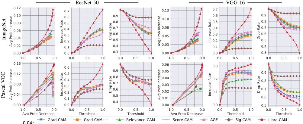
Quantitative attribution quality Figure 1 shows the API, APD, IR, and DR values for tested attribution maps: we evaluated the values at multiple threshold levels in [0, 1] to study their characteristics in regard to thresholding (when t = 0, we set all measures to zero). We think all attribution maps should be usable at their fullness (i.e., at t = 1), since otherwise, users need to figure out suitable thresholds. In the first plots in each dataset/network combination, we show the API versus APD plot mimicking the TPR vs. FPR plot in the ROC analysis, considering increases and decreases in class probability as true and false-positive detection of class-relevant input features, respectively. These plots were used to compute the AUC values in the subsequent results (all AUC values were computed with scaled API values to the [0, 1] range with respect to each API vs. APD plot).
The curves demonstrate that our Libra-CAM has better attribution quality (higher AUC, API, and IR; lower APD and DR) than the competing methods consistently overall threshold levels, datasets, and neural nets. An exception is AGF in the Pascal VOC/VGG-16 combination, where it shows higher IR at thresholds t ∈ [0.1, 0.2] and lower DR at t ∈ [0.1, 0.3]: however, Libra-CAM outperformed AGF at all larger thresholds. Moreover, the attribution quality of AGF was not consistent over different cases: it was the second-best in the Imagenet/VGG-16 case but one of the worst in the case of PascalVOC/ResNet-50. In Pascal VOC/ResNet-50, all methods except for Libra-CAM seemed to suffer from API drops at large threshold levels. This can be problematic for users of these methods who do not know such issues and expect to use the attribution maps as a whole.
Table 1 shows the AUC values (as described above) and other attribution quality measures without thresholding (that is, t = 1). The results show that Libra-CAM clearly outperforms the competing methods in all measures and cases, by good margins shown in the improvement row comparing Libra-CAM to the second-best cases in each quality assessment. Score-CAM was the second-best overall, except for Pascal VOC/ResNet-50 where the second-best was unclear.
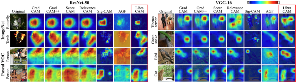
Qualitative attribution quality Figure 2 shows examples of attribution maps generated by our Libra-CAM and the competing methods. Although visual quality assessment can be subjective, Libra-CAM appears to be good at localizing the classified objects (e.g., in Butterfly and Person:top), detection of multiple objects of the same class (in Person:bottom, Tibetan terrier, and Cat), and detection of the entirety of a single object (in Green snake and Bird). The results of Grad-CAM, Grad-CAM++, Score-CAM, and Relevance-CAM were quite similar, especially the first two were almost indistinguishable. SIG-CAM's attribution maps were often quite spotty, not clearly capturing the objects (in Torch, Person:bottom, Tibetan terrier, and Green snake). AGF's attribution was noisy without enough localization in quite a few cases (in Torch, Person:top, and Person:bottom).
Ablation study To evaluate how much using references (R), reference filtering (F), and threshold calibration (C) contribute to the performance of Libra-CAM, we performed an ablation study measuring the AUC values of attribution as shown in Table 2. Comparing to each of the previous cases, we identified up to 11% (R), 30% (F), and 22% (C) quality improvement by using the components additionally.
Computation time To provide an attribution map for each input in a timely manner, efficient implementation of attribution should be an essential consideration. As shown in Table 3, our Libra-CAM can be computed in a reasonable amount of time similar to that of AGF using our GPU-based implementation.
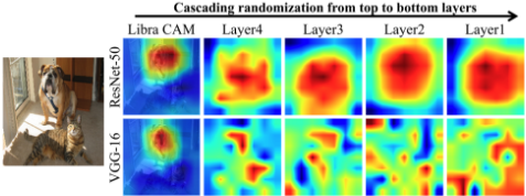
Sanity check Figure 3 shows the sensitivity of Libra-CAM following the sanity check [Adebayo et al., 2018], where attribution maps are generated while model parameters are randomized from the top to the bottom layers in a cascading fashion. The result shows that Libra-CAM is sensitive to weight perturbation and, therefore, passes the sanity check.
| Dataset | Method | ResNet-50 | VGG-16 | ||||||||
|---|---|---|---|---|---|---|---|---|---|---|---|
| AUC↑ | API↑ | APD↓ | IR↑ | DR↓ | AUC↑ | API↑ | APD↓ | IR↑ | DR↓ | ||
| Grad-CAM | 0.145 | 0.043 | 0.100 | 0.381 | 0.616 | 0.114 | 0.041 | 0.137 | 0.294 | 0.702 | |
| Grad-CAM++ | 0.145 | 0.043 | 0.100 | 0.379 | 0.618 | 0.101 | 0.037 | 0.145 | 0.278 | 0.717 | |
| Relevance-CAM | 0.163 | 0.051 | 0.099 | 0.393 | 0.603 | 0.138 | 0.052 | 0.137 | 0.304 | 0.692 | |
| ImageNet Score-CAM | 0.190 | 0.060 | 0.064 | 0.421 | 0.574 | 0.163 | 0.061 | 0.104 | 0.318 | 0.678 | |
| AGF | 0.144 | 0.042 | 0.138 | 0.350 | 0.646 | 0.154 | 0.052 | 0.135 | 0.336 | 0.660 | |
| Sig-CAM | 0.042 | 0.021 | 0.459 | 0.130 | 0.870 | 0.024 | 0.017 | 0.547 | 0.074 | 0.926 | |
| Libra-CAM | 0.273 | 0.115 | 0.034 | 0.721 | 0.276 | 0.267 | 0.129 | 0.030 | 0.705 | 0.291 | |
| Improvement | ×1.44 | ×1.92 | ×1.88 | ×1.71 | ×2.08 | ×1.64 | ×2.11 | ×3.47 | ×2.10 | ×2.27 | |
| Grad-CAM | 0.365 | 0.043 | 0.036 | 0.318 | 0.680 | 0.335 | 0.046 | 0.015 | 0.250 | 0.608 | |
| Grad-CAM++ | 0.366 | 0.043 | 0.036 | 0.320 | 0.680 | 0.328 | 0.046 | 0.019 | 0.241 | 0.659 | |
| Relevance-CAM | 0.329 | 0.032 | 0.035 | 0.316 | 0.684 | 0.197 | 0.025 | 0.044 | 0.198 | 0.657 | |
| Pascal VOC Score-CAM | 0.364 | 0.046 | 0.030 | 0.327 | 0.671 | 0.360 | 0.048 | 0.006 | 0.266 | 0.587 | |
| AGF | 0.287 | 0.037 | 0.044 | 0.422 | 0.576 | 0.388 | 0.042 | 0.017 | 0.230 | 0.557 | |
| Sig-CAM | 0.203 | 0.086 | 0.100 | 0.249 | 0.751 | 0.151 | 0.028 | 0.195 | 0.129 | 0.856 | |
| Libra-CAM | 0.428 | 0.157 | 0.001 | 0.648 | 0.351 | 0.400 | 0.060 | 0.003 | 0.313 | 0.506 | |
| Improvement | ×1.17 | ×1.83 | ×30.0 | ×1.54 | ×1.64 | ×1.03 | ×1.25 | ×2.00 | ×1.18 | ×1.10 | |
| Dataset | R | F | C | ResNet-50 | Ratio VGG-16 | Ratio | |
|---|---|---|---|---|---|---|---|
| ImageNet | 7 3 3 | 7 7 3 | 7 7 7 | 0.173 0.180 0.224 | 1.00 1.04 1.29 | 0.158 0.176 0.223 | 1.00 1.11 1.41 |
| 7 | 7 | 0.386 | 1.00 1.04 | 0.383 0.390 | 1.00 | ||
| 3 | 3 | 3 | 0.273 | 1.58 | 0.267 | 1.69 | |
| Pascal VOC | 7 | ||||||
| 3 | 7 | 7 | 0.403 | 1.03 | |||
| 3 | 3 | 7 | 0.408 | 1.06 | 0.397 | 1.04 | |
| 3 | 3 | 3 | 0.428 | 1.11 | 0.400 | 1.04 |
| Network | Method | ResNet-50 | VGG-16 |
|---|---|---|---|
| ImageNet | Grad-CAM Grad-CAM++ Relevance-CAM Score-CAM AGF Sig-CAM Libra-CAM | 0.042 (0.002) 0.034 (0.002) 0.046 (0.003) 15.234 (0.325) 0.410 (0.017) 9.290 (0.244) 0.263 (0.007) | 0.017 (0.001) 0.027 (0.001) 0.058 (0.002) 1.700 (0.014) 0.154 (0.004) 8.533 (0.184) 0.291 (0.006) |
| Pascal VOC | Grad-CAM Grad-CAM++ Relevance-CAM Score-CAM AGF Sig-CAM Libra-CAM | 0.033 (0.002) 0.033 (0.002) 0.034 (0.002) 13.959 (0.892) 0.421 (0.030) 8.944 (0.223) 0.168 (0.004) | 0.020 (0.001) 0.026 (0.001) 0.058 (0.001) 2.355 (0.021) 0.155 (0.004) 8.341 (0.192) 0.146 (0.002) |
5 RelatedWork
Input saliency methods Output changes due to input perturbation provide useful information for attribution [Erhan et al., 2009]. [Oquab et al., 2014] attributed each pixel for a class by the class score averaged over image patches containing the pixel. [Zeiler and Fergus, 2014] used the deconvnet and perturbed images with occluding patches to find out parts of the image that lead to strong activation. LIME [Ribeiro et al., 2016] used a local model to explain the prediction of the classifier, while SHAP [Lundberg and Lee, 2017] approximated the Shapley values for input attribution. Recently, EMP [Fong and Vedaldi, 2017] used edited images to learn the focus areas of a predictor. I-GOS [Qi et al., 2020] extended EMP achieving better convergence. To reduce computation, RISE [Petsiuk et al., 2018] used a linear combination of random masks, while XRAI [Kapishnikov et al., 2019] used over-segmented images testing the relevance of growing regions.
Gradient-based methods Gradients give sensitivity information of input features. Guided Backpropagation [Springenberg et al., 2015] modified gradients using the deconvnet for better attribution of input features. Integrated Gradients [Sundararajan et al., 2017] used an average of gradients along a path between the input and a baseline image, whereas Guided Integrated Gradients [Kapishnikov et al., 2021] aimed to remove the noise accumulation along the path. DeepLIFT [Shrikumar et al., 2017] decomposed the output by backpropagation and assigned contribution scores to each neuron according to the difference to a reference activation.
Relevance-propagation methods Layer-wise relevance propagation (LRP) [Bach et al., 2015] suggested a way of backpropagating the output (relevance) throughout the layers of a neural net. [Gu et al., 2018] suggested a modification to LRP at the final layer so that the attribution will reflect class information better. RAP [Nam et al., 2020] added a new feature to LRP to consider relevant and irrelevant attribution separately. AGF [Gur et al., 2021] suggested an integration of gradient-based and attribution-propagation methods.
Activation-based methods These methods make use of values from intermediate layers for attribution. GradCAM [Selvaraju et al., 2017] generalized CAM [Zhou et al., 2016] so that attribution can be done without explicit modification of the neural network, where GradCAM++ [Chattopadhay et al., 2018] tried to improve its channel weight computation. Score-CAM [Wang et al., 2020] and Relevance-CAM [Lee et al., 2021] replaced gradient information with classification scores of channel-masked images and relevance scores from Contrastive LRP [Gu et al., 2018], respectively, to avoid issues from noisy gradients. SIG-CAM [Zhang et al., 2021] suggested a weighted GradCAM fine-tuned with I-GOS [Qi et al., 2020].
6 Conclusion
We suggested Libra-CAM, a new CAM-style feature attribution method based on the best linear approximation of convolutional deep neural nets. In addition to the base form of Libra-CAM that is naturally derived from the approximation, we have discussed reference selection, library creation, and threshold calibration, all of which have been contributed to Libra-CAM to outperform the existing attribution methods we have tried. Libra-CAM is also computable in a timely manner using our GPU-based implementation. We expect Libra-CAM will be applicable in many application domains where convolutional neural nets are available.
Acknowledgements
This research was supported by Basic Science Research Program through the National Research Foundation of Korea (NRF) funded by the Ministry of Education (NRF2018R1D1A1B07051383), and by the MSIT (Ministry of Science and ICT), Korea, under the ITRC(Information Technology Research Center) support program (IITP-2020-001749) supervised by the IITP (Institute of Information & Communications Technology Planning & Evaluation).
@inproceedings{ijcai2022p442,
  title     = {Libra-CAM: An Activation-Based Attribution Based on the Linear Approximation of Deep Neural Nets and Threshold Calibration},
  author    = {Lee, Sangkyun and Han, Sungmin},
  booktitle = {Proceedings of the Thirty-First International Joint Conference on
               Artificial Intelligence, {IJCAI-22}},
  publisher = {International Joint Conferences on Artificial Intelligence Organization},
  editor    = {Luc De Raedt},
  pages     = {3185--3191},
  year      = {2022},
  month     = {7},
  note      = {Main Track},
  doi       = {10.24963/ijcai.2022/442},
  url       = {https://doi.org/10.24963/ijcai.2022/442},
}
TY - CPAPER TI - Libra-CAM: An Activation-Based Attribution Based on the Linear Approximation of Deep Neural Nets and Threshold Calibration AU - Lee, Sangkyun AU - Han, Sungmin T2 - Proceedings of the Thirty-First International Joint Conference on Artificial Intelligence, IJCAI-22 PB - International Joint Conferences on Artificial Intelligence Organization PY - 2022 SP - 3185 EP - 3191 DO - 10.24963/ijcai.2022/442 UR - https://doi.org/10.24963/ijcai.2022/442 ER -Copied
Machine-readable versions of this paper, for tools and AI agents:





