Forgiving Debt in Financial Network Games

1 Introduction

A financial system comprises a set of institutions, such as banks, that engage in financial transactions. The interconnections showing the liabilities (financial obligations or debts) among the banks can be represented by a network, where the nodes correspond to banks and the edges correspond to liability relations. Each bank has a fixed amount of external assets (not affected by the network) which are measured in the same currency as the liabilities. A bank's total assets comprise its external assets and its incoming payments, and may be used for (outgoing) payments to its lenders. If a bank's assets are not enough to cover its liabilities, that bank will be in default and the value of its assets will be decreased (e.g., by liquidation); the extent of this decrease is captured by default costs and essentially implies that the corresponding bank will have only a part of its total assets available for making payments.

∗Corresponding author

On the liquidation day (a.k.a. clearing), each bank in the system has to pay its debts in accordance with three principles of bankruptcy law (see, e.g., [Eisenberg and Noe, 2001]): i) absolute priority, i.e., banks with sufficient assets pay their liabilities in full, ii) limited liability, i.e., banks with insufficient assets to pay their liabilities are in default and pay all of their assets to lenders, subject to default costs, and iii) proportionality, i.e., in case of default, payments to lenders are made in proportion to the respective liability. Payments that satisfy the above properties are called clearing payments and maximal clearing payments, i.e., ones that point-wise maximize all corresponding payments, are known to exist and can be efficiently computed [Rogers and Veraart, 2013].

The total liquidity of a financial system is measured by the sum of payments made at clearing, and is a natural metric for the well-being of the system [Lee, 2013]. Financial authorities, e.g., governments or other regulators, wish to keep the systemic liquidity as high as possible and they might interfere, if their involvement is necessary and would considerably benefit the system. For example, in the not so far past, the Greek government (among others) took loans in order to bailout banks that were in danger of defaulting, to avert collapse. In this work, we study the possibility of a financial regulating authority performing cash injections (i.e., bailouts) to selected bank(s) and/or forgiving debts selectively, with the aim of maximizing the total liquidity of the system. Similarly to cash injections, it is a fact that debt removal can have a positive effect on systemic liquidity. Indeed, the existence of default costs can lead to the counter-intuitive phenomenon whereby removing a debt/edge from the financial network might result in increased money flow, e.g., if the corresponding borrower avoids default costs because of the removal.

Even more surprising than the increase of liquidity by the removal of debts, is the fact that the removal of an edge from borrower b to lender l might result in l receiving more incoming payments, e.g., if b avoids default costs and there is an alternative path in the network where money can flow from b to l. This motivates the definition of an edge-removal game on financial networks, where banks act as strategic agents who wish to maximize their total assets and might intentionally give-up a part of their due incoming payments towards this goal. This strategic consideration is meaningful both in the context where a financial authority performs cash injections or not. We consider the existence, quality, and computation of equilibria that arise in such games.

1.1 Our Contribution

We consider computational problems related to maximizing systemic liquidity, when a financial authority can modify the network by appropriately removing debt, or by injecting cash into selected agents. We also consider financial network games where agents can choose to forgive incoming debts.

We show how to compute the optimal cash injection policy in polynomial time when there are no default costs, by solving a linear program; the problem is NP-hard when non-trivial default costs apply. As our LP-based algorithm requires knowledge of the available budget and leads to non-monotone payments, we study the approximation ratio of a greedy cash injection policy. Regarding debt removal, we prove that finding the set of liabilities whose removal maximizes systemic liquidity is NP-hard, and so are relevant optimization problems.

Regarding edge-removal games, with or without bailout, we study the existence and the quality of Nash equilibria, while also addressing computational complexity questions. Apart from arguing about well-established notions, such as the Price of Anarchy and the Price of Stability, we introduce the notion of the Effect of Anarchy (Stability, respectively) as a new measure on the quality of equilibria in this setting.

1.2 RelatedWork

Our model is based on the seminal work of Eisenberg and Noe [2001] who introduced a widely adopted model for financial networks, assuming debt-only contracts and proportional payments. This was later extended by Rogers and Veraart [2013] to allow for default costs. Additional features have been since introduced, see e.g., [Schuldenzucker et al., 2020] and [Papp and Wattenhofer, 2020]. We follow the model of Eisenberg and Noe and consider proportional payments; we note that a recent series of papers introduced different payment schemes [Bertschinger et al., 2020; Papp and Wattenhofer, 2020; Kanellopoulos et al., 2021].

When the financial regulator has available funds to bailout each bank of the network, Jackson et al. [2020] characterize the minimum bailout budget needed to ensure systemic solvency and prove that computing it is an NP-hard problem. When the financial authority has limited bailout budget, Demange [2018] proposes the threat index as a means to determine which banks should receive cash during a default episode and suggests a greedy algorithm for this process. Egressy and Wattenhofer [2021] focus on how central banks should decide which insolvent banks to bailout and formulate corresponding optimization problems. Dong et al. [2021] introduce an efficient greedy-based clearing algorithm for an extension of the Eisenberg-Noe model, while also studying bailout policies when banks in default have no assets to distribute. We note that the problem of injecting cash (as subsidies) in financial networks has been studied (in a different context) in microfinance markets [Irfan and Ortiz, 2018].

Further work includes [Schuldenzucker and Seuken, 2020] that considers the incentives banks might have to approve the removal of a set of liabilities forming a directed cycle in the financial network, while [Schuldenzucker et al., 2017] considers the complexity of finding clearing payments when Credit Default Swap (3-party) contracts are allowed. In a similar spirit, [Ioannidis et al., 2021] studies the clearing problem from the point of view of irrationality and approximation strength, while [Papp and Wattenhofer, 2021] studies which banks are in default, and how much of their liabilities these defaulting banks can pay.

2 Preliminaries

A financial network N = (V,E) consists of a set V = {v1, . . . , vn} of n banks and a set E containing directed edge (vi, vj) among these banks, where each bank vi initially has some non-negative external assets ei corresponding to income received from entities outside the financial system. Banks have payment obligations, i.e., liabilities, among themselves. In particular, a debt contract creates a liability lij of bank vi (the borrower) to bank vj (the lender); we assume that lij ≥ 0 and lii = 0. Note that lij > 0 and lji > 0 may both hold simultaneously. Also, let Li = ∑j lij be the total liabilities of bank vi. Banks with sufficient funds to pay their obligations in full are called solvent banks, while ones that cannot are in default. Then, the relative liability matrix Π ∈ Rn×n is defined by

Let pij denote the actual payment 1 from vi to vj; we assume that pii = 0. These payments define a payment matrix P = (pij) with i, j ∈ [n], where by [n] we denote the set of integers {1, . . . , n}. We denote by pi = ∑j∈[n] pij the total outgoing payments of bank vi. A bank in default may need to liquidate its external assets or make payments to entities outside the financial system (e.g., to pay wages). This is modeled using default costs defined by values α, β ∈ [0, 1]. A bank in default can only use an α fraction of its external assets and a β fraction of its incoming payments (the case without default costs is captured by α = β = 1). The absolute priority and limited liability regulatory principles, discussed in the introduction, imply that a solvent bank must repay all its obligations to all its lenders, while a bank in default must repay as much of its debt as possible, taking default costs also into account. Summarizing, it must hold that pij ≤ lij and, furthermore, P = Φ(P), where

Payments P that satisfy these constraints are called clearing payments. Proportional payments have been frequently studied in the financial literature (e.g., in [Demange, 2018; Eisenberg and Noe, 2001; Rogers and Veraart, 2013]). Given clearing payments P, in order to satisfy proportionality, each pij must also satisfy pij = lij when vi is solvent, and pij = (αei + β ∑j∈[n] pji) πij , when vi is in default.

1 Note that the actual payment need not equal the liability, i.e., the payment obligation.

Given clearing payments P, the total assets ai(P) of bank vi are defined as the sum of external assets plus incoming payments, i.e.,

Maximal clearing payments, i.e., ones that point-wise maximize all corresponding payments (and hence total assets), are known to exist [Eisenberg and Noe, 2001; Rogers and Veraart, 2013] and can be computed in polynomial time.

We measure the total liquidity of the system (also refered to as systemic liquidity) F(P) as the sum of payments traversing through the network, i.e.

We assume that there exists a financial authority (a regulator) who aims to maximize the systemic liquidity. In particular, the regulator can decide to remove certain debts (edges) from the network or inject cash to some bank(s). In the latter case, we assume the regulator has a total budget M available in order to perform cash injections to individual banks. We sometimes refer to the total increased liquidity, ∆F, (as opposed to total liquidity) which measures the difference in the systemic liquidity before and after the cash injections. A cash injection policy is a sequence of pairs of banks and associated transfers ((i1, t1), (i2, t2), . . . (iL, tL)) ∈ (V ×R)L, such that the regulator gives capital t1 to bank i1, t2 to bank i2, etc. These actions naturally define two corresponding optimization problems on the total (increased) liquidity, i.e., optimal cash injection and optimal debt removal.

We will also find useful the notion of the threat index 2 , µi, of bank vi, which captures how many units of total increased liquidity will be realized if the financial authority injects one unit of cash into bank vi's external assets [Demange, 2018]; a unit of cash represents a small enough amount of money so that the set of banks in default would not change after the cash injection. We remark that for the maximum total increased liquidity it holds ∆F ≤ M · µmax, where µmax is the maximum threat index. Naturally, the threat index of solvent banks is 0, while the threat index of banks in default will be at least 1. Formally, the threat index is defined as

where D = {j|aj(P) < Lj} is the set of banks in default. 3

2 The term threat index aims to capture the "threat" posed to the network by a decrease in a bank's cash-flow or even the bank's default; this index can be thought of as counting all the defaulting creditors that would follow a potential default of the said bank.

3 We note that threat indexes can be efficiently computed.

An Example. Figure 1 provides an example of a financial network, inspired by an example in [Demange, 2018]. The clearing payments are as follows: p21 = 4.4, p32 = 3.2, and p43 = p45 = 1, implying that banks v2, v3 and v4 are in default. We assume that there are no default costs, i.e., α = β = 1. The threat indexes are computed as follows: µ1 = µ5 = 0, µ2 = 1 + µ1, µ3 = 1 + µ2, and µ4 = 1 + 12 µ3 + 12 µ5, implying that µ3 = µ4 = 2, µ2 = 1, while µ1 = µ5 = 0.

3 Computing and Approximating Optimal Outcomes

In this section we present algorithmic and complexity results regarding the problems of computing optimal cash injection (see Section 3.1) and debt removal (Section 3.2) policies. Note that we omit referring to default costs in our statements for those results that hold when α = β = 1.

3.1 Optimal Cash Injections

We begin with a positive result about computing the optimal cash injection policy when default costs do not apply.

Theorem 1. Computing the optimal cash injection policy can be solved in polynomial time.

Proof. The proof follows by solving a linear program that computes the optimal cash injections and accompanying payments. In particular, we denote by xi the cash injection to bank i and by pij the payment from i to j. We aim to maximize the total liquidity, i.e., the total payments, subject to satisfying the limited liability and absolute priority principles. Recall that M is the budget, lij is the liability of i to j, ei is the external assets of bank i, and πij is the (i, j)-th entry of relative liability matrix Π.

The first constraint corresponds to the budget constraint, while the second and third sets of constraints guarantee that no bank pays more than her total assets or more than a given liability; hence, the limited liability principle is satisfied. It remains to argue about the absolute priority principle, i.e., a bank can pay strictly less than her total assets only if she fully repays all outstanding liabilities.

Consider the optimal solution corresponding to a vector of cash injections and payments pij; we will show that this solution satisfies the absolute priority principle as well. We distinguish between two cases depending on whether a bank is solvent or in default. In the first case, consider a solvent bank i, i.e., xi + ei + ∑j pji ≥ Li, for which pik < lik for some bank k. By replacing pik with p′ik = lik, we obtain another feasible solution that strictly increases the objective function; a contradiction to the optimality of the starting solution. Similarly, consider a bank i with xi+ei+∑j pji < Li for which ∑j pij < xi + ei + ∑j pji. Then, there necessarily exists a bank k for which pik < (xi + ei + ∑j pji) · πik and it suffices to replace pik with p′ik = (xi + ei + ∑j pji) · πik to obtain another feasible solution that, again, strictly increases the objective function. Hence, we have proven that the optimal solution to the linear program satisfies the absolute priority principle and the claim follows by providing each bank i a cash injection of xi.

Note that the optimal policy does not satisfy certain desirable properties. In particular, as observed in [Demange, 2018], cash injections are not monotone with respect to the budget. To see that, consider the financial network in Figure 1 and note that when M = 0.5, the optimal policy would give all available budget to bank v3, while under an increased budget of 1.6, the entire budget would be allocated to v4, hence v3 would get nothing. Furthermore, our LP-based algorithm crucially relies on knowledge of the available budget.

In an attempt to alleviate these undesirable properties, we turn our attention to efficiently approximating the optimal cash injection policy by a natural and intuitive greedy algorithm, and we compute its approximation ratio under a limited budget, when we care about the total increased liquidity.

Definition 1 (GREEDY and its approximation ratio). According to GREEDY (the Greedy cash injection policy), banks receive their cash injections in sequence, so that ik, for k = 1, . . . ,L, is the bank with the highest threat index after the cash injection at round k - 1 (round 0 is defined to be the starting configuration), while tk is the minimum amount that would cause a change in the vector of threat indexes at the time it is transferred (it would lead to some previously defaulting bank to become solvent). 4 This process is repeated until the budget runs out.

The approximation ratio of GREEDY shows how smaller the total increased liquidity (or money flow) can be, compared to the optimal total increased liquidity, and is computed as

where the minimum is computed over all possible networks and budgets.

Let us revisit the example in Figure 1, assuming a budget M = 1.6. Initially banks v3 and v4 have the highest threat index of µ3 = µ4 = 2 compared to µ1 = µ5 = 0, and µ2 = 1.

4 Without loss of generality we assume ties are broken in favor of the smallest index.

We can assume 5 that bank v3 would receive the first cash injection (i1 = v3) and in fact this will be equal to t1 = 0.8. Indeed, a cash injection of 0.8 to v3 will result in v3 becoming solvent (notice that v3 receives 1 from v4), while a smaller cash injection would not impose any change on the threat index vector. At this stage, the threat index of each bank is as follows µ′1 = µ′3 = µ′5 = 0 and µ′2 = µ′4 = 1. At this round, i2 = v2 would receive the remaining budget of t2 = 0.8. Hence, the total increased liquidity achieved by GREEDY at this instance is ∆FGreedy = 2.4 (t1 will traverse edges (v3, v2) and (v2, v1), while t2 will traverse edge (v2, v1)). However, the optimal cash injection policy is to inject the entire budget M = 1.6 to bank v4 resulting in ∆FOPT = 3.2. Therefore, this instance reveals RGREEDY ≤ 2.4 3.2 = 3/4.

Theorem 2. GREEDY's approximation ratio is at most 3/4. For inputs satisfyingM ≤ t1 µv µv-1 , this ratio is tight.

We conclude this section with some hardness results.

Theorem 3. The following problems are NP-hard: a) compute the optimal cash injection policy under the constraint of integer payments, b) compute the optimal cash injection policy with default costs α ∈ [0, 1) and β ∈ [0, 1], and c) compute the minimum budget so that a given agent becomes solvent, with default costs α ∈ [0, 1/2) and β ∈ [0, 1].

Proof Sketch. We only present here a sketch of the proof of parts b and c; both follow by a reduction from the PARTITION problem, a well-known NP-complete problem. Recall that in PARTITION, an instance I consists of a set X of positive integers {x1, x2, . . . , xk} and the question is whether there exists a subset X′ of X such that ∑i∈X′ xi = ∑i/∈X′ xi = 1 2 ∑i∈X xi.

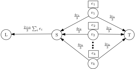
The reduction works as follows. Starting from I, we build an instance I ′ by adding an agent vi for each element xi ∈ X and allocating an external asset of ei = xi to vi; we also include three additional agents S, T and L. Each agent vi has liability equal to 4ei 3 to S and equal to 2ei 3 to T, while S has liability 2+α 3 ∑i ei to L; see also Figure 2. We assume the presence of default costs α ∈ [0, 1), and β ∈ [0, 1], while the budget is M = 12 ∑i ei; clearly, the reduction requires polynomial-time.

5 This is consistent to our tie breaking assumption that favors the least index.

Part b follows by first showing that if I is a yes-instance for PARTITION, then the total liquidity is F = 5α+10 6 ∑i ei, as well as showing that any cash injection policy that leads to a total liquidity of at least 5α+10 6 ∑i ei leads to a solution for instance I of PARTITION.

Part c follows by arguing that any cash injection policy with a budget of 1 2 ∑i ei that can make agent S solvent leads to a solution for instance I when the default costs are α ∈ [0, 1/2), β ∈ [0, 1], and vice versa.

3.2 Optimal Debt Removal

In this section, we focus on maximizing systemic liquidity by appropriately removing edges/debts. As an example, consider again Figure 1, where the central authority can increase systemic liquidity by removing the edge between v4 and v5.

Theorem 4. The problem of computing an edge set whose removal maximizes systemic liquidity is NP-hard.

We note that the objective of systemic solvency, i.e., guaranteeing that all agents are solvent, can be trivially achieved by removing all edges. However, adding a liquidity target, makes this problem more challenging.

Theorem 5. In networks with default costs, the following three problems are NP-hard. Compute an edge set whose removal: a) ensures systemic solvency and maximizes systemic liquidity, b) ensures systemic solvency and minimizes the amount of deleted liabilities, and c) guarantees that a given agent is no longer in default and minimizes the amount of deleted liabilities.

4 The Edge-Removal Game

In this section, we consider the case of strategic agents who have the option to forgive debt. Consider a financial network N of n banks who act strategically. The strategy set of a bank is the power set of its incoming edges and a strategy denotes which of its incoming edges that bank will remove, thus erasing the corresponding debt owed to itself. The edge-removal game can be defined with and without cashinjections. A given strategy vector will result in realized payments through maximal clearing payments including possible cash injections through a predetermined cash injection policy. Our results hold for both the optimal policy and GREEDY.

A bank is assumed to strategize over its incoming edges in order to maximize its utility, i.e., its total assets, where we remark that a possible cash injection can be seen as increasing one's external assets. The objective of the financial authority is to maximize the total liquidity of the system, i.e., the social welfare is the sum of money flows that traverse the network.

We consider the central notion of Nash equilibrium strategy profile, under which no bank can unilaterally increase its utility by changing strategy; let Seq denote the set of strategy profiles at equilibrium. The inefficiency of Nash equilibria in terms of liquidity is measured by the Price of Anarchy (Stability, respectively) which is equal to optimal systemic liquidity, denoted by FOPT , over that of the worst (best, respectively) pure Nash equilibrium. Note that the optimal systemic liquidity corresponds to the maximal one when the financial authority can dictate everyone's actions (edge-removals).

The Price of Anarchy/Stability notions provide indications regarding the extent to which the individual objectives of the banks and the objective of the regulator are (not) aligned. We, here, introduce a new notion that we use to measure the discrepancy between the systemic liquidity of the original network (no edge removal), denoted by FN, and that of worst (best) Nash equilibrium. We call this the Effect of Anarchy, (Stability, respectively) and define it as follows.

We investigate properties of Nash equilibria in the edgeremoval game with respect to their existence and quality, while we also address computational complexity questions under different assumptions on whether default costs and/or cash injections apply. Our results on the Effect of Anarchy of edge removal games imply that, rather surprisingly, in the presence of default costs even the worst Nash equilibrium can be arbitrarily better than the original network in terms of liquidity. However, the situation is reversed in the absence of default costs, where we observe that the original network can be considerably better in terms of liquidity than the worst equilibrium; in line with similar Price of Anarchy results. We begin with some results for the basic case, that is, without default costs; recall that we do not refer to default costs in the statements for results holding for α = β = 1.

Our first result exploits the fact that, for edge-removal games without cash injections, the strategy profile where all edges are preserved is a (not necessarily unique) Nash equilibrium.

Theorem 6. Edge-removal games without cash injections always admit Nash equilibria.

Theorem 7. In edge-removal games without cash injections, the Effect of Anarchy is unbounded and the Effect of Stability is at most 1.

Our next result shows that Nash equilibria may not exist once we allow for cash injections.

Theorem 8. There is an edge-removal game with cash injections that does not admit Nash equilibria.

Theorem 9. The Price of Stability in edge-removal games (with or without cash injections) is unbounded.

Theorem 10. The Effect of Anarchy in edge-removal games with cash injections is at least n - 1.

Theorem 11. The Effect of Stability in edge-removal games with cash injections is Ω(n).

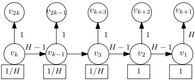
Proof. Consider the network in Figure 3 where the budget M = 1, k = n/2 and H is arbitrarily larger than k. We start by noticing that µ1 = 1, while for i = 2, . . . , k, it holds that µi = 1 + H-1 H µi-1 ≈ 1 + µi-1, for sufficiently large H; all other banks are solvent. Hence, the optimal total liquidity is achieved when vk receives the entire budget of M = 1

as a cash injection, and is roughly kM = n/2, when H is sufficiently large.

We now claim that under any Nash equilibrium, v2 will receive the budget and all edges (vi, vi-1) for i ∈ {3, . . . , k} are removed. This would complete the proof, as the total liquidity would be at most 1H (k-2)+2+2 ≤ 5. We now prove this claim. Consider any equilibrium and observe that vi, for i = k + 1, . . . , 2k, must have their unique incoming edge present. Now, assume for a contradiction that some bank vi with i ∈ {3, . . . , k} gets a cash injection; this implies that the edge (vi, vi-1) is present as, otherwise, the result holds trivially. Then, bank vi-1 has total assets 1 - 1/H2 + ei-1, but can increase them to 1 + ei-1 by strategically removing its incoming edge. So, under any Nash equilibrium, either v2 or v1 receives a cash injection. In the former case, where edge (v2, v1) is present, a1 = 3-2/H, while the assets of v1 would be 2 if it removed its incoming edge and received the cash injection.

So far, we have proven that v2 gets the cash injection and it remains to show no other edge (vi, vi-1) for i ∈ {3, . . . , k} exists in a Nash equilibrium. Now, observe that if such an edge exists, then neighboring edges on the horizontal path cannot exist as that would contradict that v2 gets the cash injection. Then, when i > 4, bank vi-2 would have an incentive to add edge (vi-1, vi-2), thus, making bank vi the recipient of the budget (for both optimal and greedy) and strictly increase its own total assets. The cases i ∈ {3, 4} can be easily ruled out as well. Our proof is complete.

We now present a series of results for the case where default costs exist, but cash injections are not allowed. Contrary to the case with neither default costs nor cash injections, we show that a Nash equilibrium is no longer guaranteed to exist; the next result is complementary to Theorem 8.

Theorem 12. There is an edge-removal game with default costs but without cash injections that does not admit Nash equilibria.

For some restricted topologies, however, the existence of Nash equilibria is guaranteed; in particular, keeping all edges is a Nash equilibrium.

Theorem 13. Edge-removal games with default costs but without cash injections always admit Nash equilibria if the financial network is a tree or a cycle.

The following result demonstrates that the positive impact of (individually benefiting) edge removals dominates the negative impact of reducing the number of edges through which money can flow, hence, edge removals are in line with the regulator's best interest too.

Lemma 1. Edge-removal games with default costs but no cash injections satisfy the following: given any network and any strategy profile, any unilateral removal of any edge(s) that weakly improves the total assets of the corresponding bank, also weakly improves the total assets of every other bank in the network. Consequently, the total liquidity of the system is increased.

In fact, the systemic liquidity of even the worst Nash equilibrium can be arbitrarily higher than at the original network. To see this, consider the network in the proof of Theorem 14, which admits a unique Nash equilibrium with arbitrarily higher total liquidity than that of the original network.

Theorem 14. When default costs apply but there are no cash injections, the Effect of Stability is arbitrarily close to 0.

Proof. Consider a network with n nodes, v1, . . . , vn, and edges (vi, vi+1), for i = 1, . . . , n-1, as well as edge (v1, vn), all with unit liability. Only bank v1 has one unit of external asset, while we assume default costs α = β = ϵ for some arbitrary small positive constant ϵ.

If no edge is removed, then all banks except vn are in default and the following payments are realized: p12 = p1n = ϵ/2 and pi,i+1 = ϵ · pi-1,i = ϵi /2. The systemic liquidity is then FN = ϵ/2 + ∑n-1 i=1 ϵi 2 < ϵ 1-ϵ . On the other hand, the unique Nash equilibrium is achieved when vn removes the edge pointing from v1 to itself. The systemic liquidity in this case is n - 1, and the proof follows.

We conclude with our results on computational complexity for the setting with default costs.

Theorem 15. In edge-removal games with default costs, the following problems are NP-hard: a) decide whether a Nash equilibrium exists or not, b) compute a Nash equilibrium, when it is guaranteed to exist, c) compute a best-response strategy, and d) compute a strategy profile that maximizes systemic liquidity.

5 Conclusions

We considered problems arising in financial networks, when a financial authority wishes to maximize the total liquidity either by injecting cash or by removing debt. We also studied the setting where banks are rational strategic agents that might prefer to forgive some debt if this leads to greater utility, and we analyzed the corresponding games with respect to properties of Nash equilibria. In that context, we also introduced the notion of the Effect of Anarchy (Stability, respectively) that compares the liquidity in the initial network to that of the worst (best, respectively) Nash equilibrium.

Our work leaves some interesting problems unresolved. Given the computational hardness of some of the optimization problems, it makes sense to consider approximation algorithms. From the game-theoretic point of view, one can also consider the problems from a mechanism design angle, i.e., to design incentive-compatible policies where banks weakly prefer to keep all incoming liabilities.