
Initializing Then Refining: A Simple Graph Attribute Imputation Network
Proceedings of the Thirty-First International Joint Conference on Artificial Intelligence. Main Track. Pages 3494-3500.
https://doi.org/10.24963/ijcai.2022/485
Keywords
- Machine Learning: Multi-view learning
- Machine Learning: Representation learning
- Machine Learning: Self-supervised Learning
- Machine Learning: Autoencoders
Abstract
Representation learning on the attribute-missing graphs, whose connection information is complete while the attribute information of some nodes is missing, is an important yet challenging task. To impute the missing attributes, existing methods isolate the learning processes of attribute and structure information embeddings, and force both resultant representations to align with a common in-discriminative normal distribution, leading to inaccurate imputation. To tackle these issues, we propose a novel graph-oriented imputation framework called initializing then refining (ITR), where we first employ the structure information for initial imputation, and then leverage observed attribute and structure information to adaptively refine the imputed latent variables. Specifically, we first adopt the structure embeddings of attribute-missing samples as the embedding initialization, and then refine these initial values by aggregating the reliable and informative embeddings of attribute-observed samples according to the affinity structure. Specially, in our refining process, the affinity structure is adaptively updated through iterations by calculating the sample-wise correlations upon the recomposed embeddings. Extensive experiments on four benchmark datasets verify the superiority of ITR against state-of-the-art methods.
- [Chen et al., 2019] Lei Chen, Shunwang Gong, Joan Bruna, and Michael M. Bronstein. Attributed random walk as ma- trix factorization. In NeurIPS Workshop, 2019.
- [Chen et al., 2022] Xu Chen, Siheng Chen, Jiangchao Yao, Huangjie Zheng, Ya Zhang, and Ivor W. Tsang. Learning on attribute-missing graphs. IEEE TPAMI, 44(2):740-757, 2022.
- [Gao et al., 2019] Chen Gao, Xiangnan He, Dahua Gan, Xi- angning Chen, Fuli Feng, Yong Li, TatSeng Chua, and De- peng Jin. Neural multi-task recommendation from multi- behavior data. In ICDE, page 1554-1557, 2019.
- [Grover and Leskovec, 2016] Aditya Grover and Jure Leskovec. node2vec: Scalable feature learning for networks. In KDD, pages 855-864, 2016.
- [Hamilton et al., 2017] William L. Hamilton, Zhitao Ying, and Jure Leskovec. Inductive representation learning on large graphs. In NeurIPS, pages 1024-1034, 2017.
- [Hassani and Ahmadi, 2020] Kaveh Hassani and Amir Ho- sein Khas Ahmadi. Contrastive multi-view representation learning on graphs. In ICML, pages 4116-4126, 2020.
- [Hu et al., 2017] Pengwei Hu, Keith C. C. Chan, and Tiantian He. Deep graph clustering in social network. In WWW, pages 1425-1426, 2017.
- [Hu et al., 2019] Liang Hu, Songlei Jian, Longbing Cao, Zhiping Gu, Qingkui Chen, and Artak Amirbekyan. Hers: Modeling influential contexts with heterogeneous relations for sparse and cold-start recommendation. In AAAI, pages 3830-3837, 2019.
- [Huang et al., 2019] Xiao Huang, Qingquan Song, Yuening Li, and Xia Hu. Graph recurrent networks with attributed random walks. In KDD, pages 732-740, 2019.
- [Kingma and Welling, 2014] Diederik P. Kingma and Max Welling. Auto-encoding variational bayes. In ICLR, 2014.
- [Kipf and Welling, 2016] Thomas N. Kipf and Max Welling. Variational graph auto-encoders. In ArXiv abs/1611.07308, 2016.
- [Kipf and Welling, 2017] Thomas N. Kipf and Max Welling. Semi-supervised classification with graph convolutional networks. In ICLR, 2017.
- [Liu et al., 2022] Yue Liu, Wenxuan Tu, Sihang Zhou, Xin- wang Liu, Linxuan Song, Xihong Yang, and En Zhu. Deep graph clustering via dual correlation reduction. In AAAI, 2022.
- [McCallum et al., 2000] Andrew McCallum, Kamal Nigam, Jason Rennie, and Kristie Seymore. Automating the con- struction of internet portals with machine learning. Infor- mation Retrieval, 3(2):127-163, 2000.
- [Peng et al., 2020] Zhen Peng, Wenbing Huang, Minnan Luo, Qinghua Zheng, Yu Rong, Tingyang Xu, and Jun- zhou Huang. Graph representation learning via graphical mutual information maximization. In WWW, pages 259- 270, 2020.
- [Perozzi et al., 2014] Bryan Perozzi, Rami Al-Rfou, and Steven Skiena. Deepwalk: online learning of social rep- resentations. In KDD, pages 701-710, 2014.
- [Sen et al., 2008] Prithviraj Sen, Galileo Namata, Mustafa Bilgic, Lise Getoor, Brian Gallagher, and Tina Eliassi- Rad. Collective classification in network data. Information Retrieval, 29(3):93-106, 2008.
- [Shchur et al., 2018] Oleksandr Shchur, Maximil- ian Mumme, Aleksandar Bojchevski, and Stephan Günnemann. Pitfalls of graph neural network evaluation. In ArXiv abs/1811.05868, 2018.
- [Spinelli et al., 2020] Indro Spinelli, Simone Scardapane, and Aurelio Uncini. Missing data imputation with adversarially-trained graph convolutional networks. Neu- ral Networks, 129:249-260, 2020.
- [Taguchi et al., 2021] Hibiki Taguchi, Xin Liu, and Tsuyoshi Murata. Graph convolutional networks for graphs contain- ing missing features. Future Generation Computer Sys- tems, 117:155-168, 2021.
- [Tu et al., 2021] Wenxuan Tu, Sihang Zhou, Xinwang Liu, Xifeng Guo, Zhiping Cai, En Zhu, and Jieren Cheng. Deep fusion clustering network. In AAAI, pages 9978-9987, 2021.
- [van den Berg et al., 2017] Rianne van den Berg, Thomas N Kipf, and Max Welling. Graph convolutional matrix com- pletion. In ArXiv abs/1706.02263, 2017.
- [Velickovic et al., 2018] Petar Velickovic, Guillem Cucurull, Arantxa Casanova, Adriana Romero, Pietro Liò, and Yoshua Bengio. Graph attention networks. In ICLR, 2018.
- [Wu et al., 2020] Jiapeng Wu, Meng Cao, Jackie Chi Kit Cheung, and William L. Hamilton. Temp: Temporal mes- sage passing for temporal knowledge graph completion. In EMNLP, pages 5730-5746, 2020.
- [You et al., 2020] Jiaxuan You, Xiaobai Ma, Daisy Yi Ding, Mykel J. Kochenderfer, and Jure Leskovec. Handling missing data with graph representation learning. In NeurIPS, 2020.
- [Zhang and Chen, 2020] Muhan Zhang and Yixin Chen. In- ductive matrix completion based on graph neural net- works. In ICLR, 2020.
- [Zhu et al., 2021] Yanqiao Zhu, Yichen Xu, Feng Yu, Qiang Liu, Shu Wu, and Liang Wang. Graph contrastive learning with adaptive augmentation. In WWW, pages 2069-2080, 2021.
- [Özgür Simsek and Jensen, 2008] Özgür Simsek and David D. Jensen. Navigating networks by using ho- mophily and degree. National Academy of Sciences, 105(35):12758-12762, 2008.
References were extracted automatically from the PDF and may contain errors.
Full text extracted automatically from the PDF; figures, tables and equations may differ. The PDF is the version of record.
1 Introduction
Graph data, which models the relationships between entities, is ubiquitous in practical scenarios. To handle these data, graph representation learning (GRL) has increasingly become a popular research topic and achieved remarkable success in many real-world applications such as social network analysis [Hu et al., 2017], knowledge graph completion [Wu et al., 2020], etc. It has long been proved that integrating the attribute and structure information while conducting the representation learning is essential for improving the quality of sample embeddings [Kipf and Welling, 2017;
∗Corresponding author
Chen et al., 2022]. However, in most real-world graph applications, only a small portion of samples have complete attribute information. For example, in a co-purchase graph of Amazon, consumers tend to selectively (or entirely not) provide their feedback for specific items due to privacy concerns. Consequently, graph representation learning on incompleteattribute graphs is becoming an increasingly important task.
Data imputation is a straightforward mechanism to handle incomplete-attribute graphs. Existing efforts combine the imputation-oriented machine learning techniques, e.g., matrix completion [van den Berg et al., 2017; Zhang and Chen, 2020], generative adversarial network [Spinelli et al., 2020], Gaussian mixture model (GMM) [Taguchi et al., 2021], with graph neural networks (GCNs) and propose various attributeincomplete graph representation learning methods with impressive performance. Although significant progress has been made, the performance of these methods drops drastically when handling attribute-missing graphs, i.e., graphs whose all attribute information of a specific portion of samples is missing. To solve the problem of representation learning on attribute-missing graphs, a recent advanced method named SAT [Chen et al., 2022] introduces a shared-latent space assumption to impute the attribute-missing values at the first attempt. Specifically, SAT first learns the latent representations of attribute and structure spaces independently and then conducts a distribution alignment technique to recover the unknown features of attribute-missing samples. Although SAT achieves encouraging success, when conducting the data imputation, it 1) isolates the learning processes of attribute and structure information embeddings; 2) forces both types of latent variables to align with a common in-discriminative normal distribution. Hence, the negotiation between attribute and structure information tends to get overly rigid, resulting in inaccurate imputation and less discriminative representations.
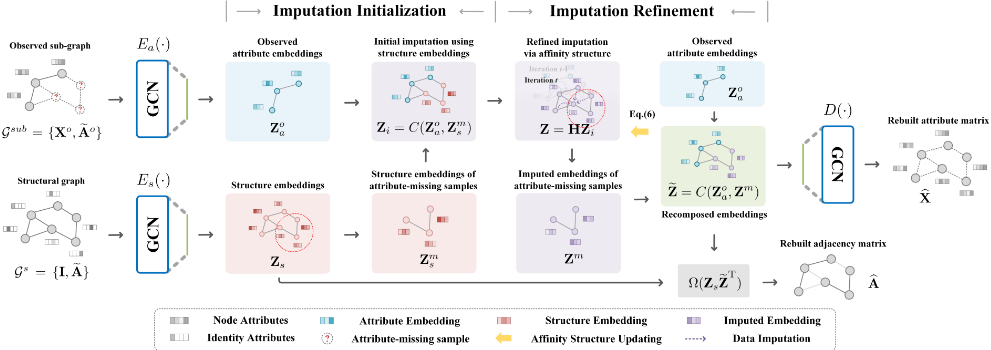
To overcome the aforementioned issues, this work proposes a novel graph attribute imputation network termed Initializing Then Refining (ITR). To forbid the adverse effect of inaccurate simple initialization and the limitation of rigid assumption, the main idea of our strategy is to make full use of the trustworthy visible information to conduct the sample embeddings for data imputation. As a consequence, on the one hand, we pick out the nodes with complete attributes and learn the sample embeddings by sufficiently combining the attribute and structure information of these samples. On the other hand, we take all the nodes and learn the sample embeddings only according to the structure information. These two processes are illustrated as the upper and underneath pathways in Fig. 1, respectively. The two mentioned operations ensure the quality of latent representations of the nodes with complete attributes, and in the meantime, provide a reasonable initialization to those nodes with missing attributes. After that, to achieve better attribute-missing graph representation learning, the structure embeddings of attribute-missing samples are taken as initial imputed variables and then refined with an adaptively updated affinity structure for embedding refinement. This is illustrated as imputation refinement in Fig. 1. Unlike the prior distribution alignment-based imputation strategy in SAT, our proposed ITR is more general and flexible, since both types of information (i.e., graph structure and node attributes) are allowed to sufficiently negotiate with each other for reliable attribute restoration. The main contributions of this paper are three-fold:
- We propose a simple yet powerful graph attribute imputation network called ITR that can jointly conduct attribute-missing graph representation learning and data imputation without any prior distribution assumption.
- We develop an initializing then refining strategy to have two-source information (i.e., graph structure and node attributes) to sufficiently negotiate with each other for accurate data imputation. By this means, more discriminative latent features could be adaptively collected and preserved to perform high-quality attribute restoration.
- Through experimental results on four benchmarks, we have demonstrated that ITR significantly and consistently outperforms the state-of-the-art counterparts on both profiling and node classification tasks.
2 RelatedWork
Graph Representation Learning. Early solutions to graph representation learning (GRL) mainly include random walkbased methods [Perozzi et al., 2014; Grover and Leskovec, 2016], which first generate the random walk sequences over the network structure properties and then utilize a Skip-Gram model to learn graph representations. These methods heavily rely on structure information and overlook other available properties in the graph, such as attribute information. More recently, since the powerful neighborhood aggregation capacity of graph neural networks (GNNs), many efforts have been made to design GNN-based representation learning methods. These methods can be approximately divided into generative/predictive learning-based methods [Kipf and Welling, 2016; Tu et al., 2021; Liu et al., 2022] and contrastive learning-based methods [Hassani and Ahmadi, 2020; Peng et al., 2020; Zhu et al., 2021]. One underlying assumption commonly adopted by these methods is that the attributes of all nodes are complete. While in real-world scenarios, they may suffer significant performance degradation when handling incomplete graphs.
Data Imputation for Incomplete Graphs. To handle incomplete graphs, data imputation has been widely integrated with machine learning techniques, such as matrix completion, generative adversarial network, and Gaussian mixture model (GMM). For example, NMTR [Gao et al., 2019] and GRAPE [You et al., 2020], the popular matrix completion methods, first regard the user-item rating matrix, users (or items), and the observed ratings as a bipartite graph, node attributes, and linkage relations, respectively. Then these methods employ a GNN-based framework to estimate the probabilities (viewed as imputed values) of absent linkage relations. More recently, GINN [Spinelli et al., 2020] first initializes the incomplete values by a binary mask matrix before network training, and then learns a graph adversarially-trained framework to perform attribute restoration. GCNMF [Taguchi et al., 2021] employs GMM to estimate the incomplete information based on the available one, and in the meanwhile, jointly optimizes GMM and GNN in a united framework. Despite their significant progress, these methods 1) are not suitable for attributemissing scenarios, or 2) disconnect the processes of data imputation and algorithm optimization. To address these issues, an advanced method called SAT [Chen et al., 2022] puts forward to unify data imputation and network learning processes into a single optimization procedure, where two-source information embeddings are learned in a decoupled scheme and then aligned with the Gaussian noise for data imputation. However, to complete the missing values, SAT isolates the learning processes of two-source information embeddings and imposes too strict a distribution assumption on the latent variables, resulting in inaccurate imputation.
3 The ProposedMethod
3.1 Notations
Given an undirected graph G = {V, E} with C classes, where V = {v1, v2, . . . , vN}, E, and N are the node set, edge set, and the number of nodes, respectively. In classic graph learning, a graph is usually characterized by its attribute matrix X ∈ RN×D and normalized adjacency matrix ˜A ∈ RN×N , where D is the node attribute dimension [Kipf and Welling, 2017]. Specially, in the attribute-missing case, with the existence of missing values, we further define V o = {vo 1 , vo 2 , . . . , voN o} and V m = {vm 1 , vm 2 , . . . , vm N m} to be the set of attribute-observed samples and the set of attribute-missing samples, respectively. Accordingly, V = V o ∪ V m, V o ∩ V m = ∅, and N = N o + N m.
3.2 Two-source Information Extraction
Unlike most current imputation-based GRL methods that perform data imputation before network training, our goal is to make full use of all trustworthy observations, i.e., attributeobserved sample information and graph structure information, to accurately impute and restore the unknown features by unifying imputation and network learning into a single optimization procedure. To this end, as shown in Fig. 1, we introduce a pseudo-Siamese architecture, which employs two identical 2-layer graph convolution networks (GCNs) as graph encoders, denoted as Ea(·) and Es(·), respectively. Here we take Ea(·) as an example to introduce the learning process of attribute-observed sample embeddings, and the learning procedure of Es(·) is similar. Specifically, the encoder Ea(·) initially accepts a given observed sub-graph G sub = {Xo , ˜Ao } as input, where Xo ∈ RN o×D and ˜Ao ∈ RN o×N o denote the observed attribute matrix and the corresponding normalized adjacency matrix. Then we compute l-th latent representations of attribute-observed samples Zo(l) a :
whereW(l) indicates the encoder network parameters of the l-th layer. σ(·) denotes the ReLU activation function. Similarly, the encoder Es(·) receives a given structural graph G s = {I, ˜A} and outputs Z(l) s , where I ∈ RN×N is identity matrix and Z(l) s denotes l-th latent representations of G s .
3.3 Initializing Then Refining
Imputation Initialization. Since only partial samples with complete attributes exist, assigning initial values to the attribute-missing ones should be considered before network training. A commonly adopted way is classic data imputation, e.g., zero-filling and mean value-filling. However, in the attribute-missing case, these tricks may introduce much irrelevant information that readily diffuses through the network, resulting in semantically biased representations. To avoid this issue, an underlying solution is to leverage the graph structure information of attribute-missing samples to implement the initial imputation in the latent space. Since the structural properties of the entire graph data are complete, the initialization for attribute-missing samples is reliable. Specifically, after obtaining two-source embeddings, i.e., Zoa ∈ RN o×d and Zs ∈ RN×d , we first select the structure embeddings of attribute-missing samples Zms ∈ RN m×d from Zs, and then combine them with observed attribute embeddings Zoa using Concat function C(·). As illustrated in Fig. 1, the concatenation operation to construct Zi is not the classic channel concatenation. In this operation, we fill the embeddings of attribute-observed samples with Zoa and the embeddings of attribute-missing samples with Zms :
| Dataset | Method | Recall@50 | NDCG@50 |
|---|---|---|---|
| Cora | Ours-Z | 34.03 | 32.08 |
| Ours-S | 34.77 | 32.95 | |
| Ours-S-A | 36.47 (1.70↑) | 34.60 (1.65↑) | |
| Citeseer | Ours-Z | 24.04 | 25.32 |
| Ours-S | 24.91 | 26.55 | |
| Ours-S-A | 26.84 (1.93↑) | 28.69 (2.14↑) |
where we denote the initially imputed embeddings as Zi ∈ RN×d . d is the embedding dimension. Please note that the position of each sample is kept unchanged within the graph. Imputation Refinement. As known, the attributes preserve the graph semantics while the structures describe the linkage relations among nodes. Hence, the discriminative capacities of both types of information exhibit differences to some extent. To verify whether our assumption holds, we compare three methods and present analyses on Cora and Citeseer. Ours-Z, Ours-S, and Ours-S-A are methods where we impute the attribute-missing part in the latent space with zero values, the structure embeddings merely, and the structureattribute embeddings, respectively. From the results in Table 1, we observe that the Ours-S method consistently outperforms the Ours-Z method but is not comparable to the OursS-A method. These results hold our expectation and clearly illustrate that although the structure embeddings could effectively serve the initial imputation task, there still exists noise in Zms that would affect the discriminative capacity of latent representations, thus leading to sub-optimal performance. To address this limitation, we try to refine the imputation process by transferring the available semantics Zoa into Zms via an affinity structure H ∈ RN×N . The intuition behind this is that the sample embeddings Zoa are reliable since the attribute information of all attribute-observed samples is complete. In this way, the semantic gap between Zoa and Zms could be narrowed to boost the expressive capacity of the whole embeddings. The above learning process can be formulated as below (i.e., a graph convolution-like operation):
where we denote the imputed embeddings as Z ∈ RN×d , here we set the affinity structure H to ˜A for initialization.
In Eq.(3), we observe that the noise information in Zms can also diffuse across the attribute-observed part, which would make the representations of Zoa less discriminative. In this circumstance, conducting the embeddings of both attribute-observed and attribute-missing samples simultaneously would undermine the quality of sample embeddings and the reconstruction accuracy of available samples, which would in turn affect the subsequent data imputation tasks and even distort the original graph. To overcome this issue, we introduce an information recomposing scheme. Firstly, we merely select the latent variables of attribute-missing samples Zm ∈ RN m×d from Z, and then recompose them with Zoa :
where we denote the recomposed embeddings as ˜Z ∈ RN×d . In our settings, the information recomposing operation replaces the adjusted embeddings of attribute-observed samples with more reliable Zoa . By doing this, we reduce the adverse effect of inaccurate information passing from the embeddings of attribute-missing samples. Moreover, the embeddings of attribute-observed samples are fixed as Zoa in the final step, as shown in Fig, 1. This provides the most trustworthy information of those samples for subsequent data imputation tasks.
It is worth noting that the initial affinity matrix H (i.e., ˜A) is not the ground truth. The errors within this matrix are twofold: 1) noisy connections. Besides inner connections within clusters, inappropriate connections could exist between clusters in the matrix; 2) missing connections. In ˜A, only the firstorder connections are recorded, the higher-order connections could be missing. Both would cause the inaccurate reconstruction of observed attributes and missing attributes. To overcome these issues, we seek to refine H to further improve the imputation quality via an affinity structure updating scheme. Specifically, we first generate a normalized selfcorrelated matrix S ∈ RN×N according to ˜Z as below:
where N(Y) = D- 1 2 Y YD- 12 Y denotes the structural normalization function, DY ∈ RN×N is the degree matrix of Y. ˜zj (˜zk) indicates the embedding of node vj (vk). Then we update the affinity structure H every t iterations via Eq.(6), and adopt it to refine the subsequent imputation process:
where α is a balanced coefficient, and we initialize it as 0.5. In this way, the affinity structure updating operation allows the network to construct the embeddings of attribute-missing samples with not only the first-order but also the higher-order connections from the original graph. Since the embeddings of attribute-observed samples become more reliable and the embeddings of attribute-missing samples become more informative, the quality of the overall graph embeddings is boosted.
| Dataset | Nodes | Edges | Dimension | Classes |
|---|---|---|---|---|
| Cora | 2708 | 5278 | 1433 | 7 |
| Citeseer | 3327 | 4228 | 3703 | 6 |
| Amac | 13752 | 245861 | 767 | 10 |
| Amap | 7650 | 119081 | 745 | 8 |
3.4 Decoding andModel Training
Finally, we directly feed ˜Z with ˜A into the denoder D(·) to complete the attribute restoration, which is formulated as:
where ˜W(l) indicates the decoder network parameters of the l-th layer. ˜Z(0) and ˜Z(2) denote the recomposed embeddings ˜Z and the rebuilt attribute matrix ̂X ∈ RN×D , respectively. The overall objective of ITR consists of two parts:
In Eq.(10), La refers to the mean square error (MSE) between the attribute-observed part of both X and ̂X. Ls refers to the binary cross-entropy (BCE) between the normalized adjacency matrix ˜A and the rebuilt adjacency matrix ̂A ∈ RN×N , where ̂A = Ω(Zs ˜ZT), Ω(·) is a sigmoid activation function. λ and γ are two balanced coefficients.
4 Experiments
4.1 Experimental Setup
Benchmark Datasets. We conduct experiments to evaluate the proposed ITR on four benchmark datasets, including Cora [McCallum et al., 2000], Citeseer [Sen et al., 2008], Amazon Computer (Amac), and Amazon Photo (Amap) [Shchur et al., 2018]. Table 2 summarizes the dataset information.
Parameters Setting. For all compared methods except for GINN [Spinelli et al., 2020] and GCNMF [Taguchi et al., 2021], the experimental results are acquired according to the paper of SAT [Chen et al., 2022]. For GINN and GCNMF methods, we run their public code by following the settings of the original papers, and then report the corresponding performance. For our proposed ITR, we strictly follow the principle of data splits as was done in SAT [Chen et al., 2022], including the split ratio of attribute-observed/-missing samples and the split ratio of train/test sets. Specifically, 1) in the profiling task, we randomly sample 40% nodes with attributes as the training set, and manually mask all attributes of the rest of 10% and 50% nodes (i.e., attribute-missing samples) as the validation set and the test set, respectively. We employ a symmetric backbone framework consisting of 4-layer GCNs and optimize it with the Adam optimization algorithm, where we set the learning rate to 1e-3. During the training phase, we transfer all samples into our ITR to restore missing attributes by merely reconstructing the attribute-observed samples (i.e., training set). After training, we directly generate the rebuilt attribute matrix over the well-trained model via forwarding propagation; 2) in the node classification task, the restored attributes are randomly split into 80% and 20% for training and testing. We train the classifier with five-fold validation for 1000 iterations and repeat the experiments 10 times. Moreover, the learning rate, the latent dimension, the dropout rate, and the weight decay are set to 1e-3, 64, 0.5, and 5e-4, respectively. Please note that we do not carefully tune these parameters for the ease of training as was done in SAT.
| Dataset | Metric | NeighAggre | VAE | GCN | GraphSage | GAT | Hers | GraphRNA | ARWMF | SAT | Ours |
|---|---|---|---|---|---|---|---|---|---|---|---|
| Cora | Recall@10 | 0.0906 | 0.0887 | 0.1271 | 0.1284 | 0.1350 | 0.1226 | 0.1395 | 0.1291 | 0.1508 | 0.1682 |
| Recall@20 | 0.1413 | 0.1228 | 0.1772 | 0.1784 | 0.1812 | 0.1723 | 0.2043 | 0.1813 | 0.2182 | 0.2369 | |
| Recall@50 | 0.1961 | 0.2116 | 0.2962 | 0.2972 | 0.2972 | 0.2799 | 0.3142 | 0.2960 | 0.3429 | 0.3647 | |
| NDCG@10 | 0.1217 | 0.1224 | 0.1736 | 0.1768 | 0.1791 | 0.1694 | 0.1934 | 0.1824 | 0.2112 | 0.2320 | |
| NDCG@20 | 0.1548 | 0.1452 | 0.2076 | 0.2102 | 0.2099 | 0.2031 | 0.2362 | 0.2182 | 0.2546 | 0.2781 | |
| NDCG@50 | 0.1850 | 0.1924 | 0.2702 | 0.2728 | 0.2711 | 0.2596 | 0.2938 | 0.2776 | 0.3212 | 0.3460 | |
| Citeseer | Recall@10 | 0.0511 | 0.0382 | 0.0620 | 0.0612 | 0.0561 | 0.0576 | 0.0777 | 0.0552 | 0.0764 | 0.0963 |
| Recall@20 | 0.0908 | 0.0668 | 0.1097 | 0.1097 | 0.1012 | 0.1025 | 0.1272 | 0.1015 | 0.1280 | 0.1548 | |
| Recall@50 | 0.1501 | 0.1296 | 0.2052 | 0.2058 | 0.1957 | 0.1973 | 0.2271 | 0.1952 | 0.2377 | 0.2684 | |
| NDCG@10 | 0.0823 | 0.0601 | 0.1026 | 0.1003 | 0.0878 | 0.0904 | 0.1291 | 0.0859 | 0.1298 | 0.1632 | |
| NDCG@20 | 0.1155 | 0.0839 | 0.1423 | 0.1393 | 0.1253 | 0.1279 | 0.1703 | 0.1245 | 0.1729 | 0.2120 | |
| NDCG@50 | 0.1560 | 0.1251 | 0.2049 | 0.2034 | 0.1872 | 0.1900 | 0.2358 | 0.1858 | 0.2447 | 0.2869 | |
| Amac | Recall@10 | 0.0321 | 0.0255 | 0.0273 | 0.0269 | 0.0271 | 0.0273 | 0.0386 | 0.0280 | 0.0391 | 0.0448 |
| Recall@20 | 0.0593 | 0.0502 | 0.0533 | 0.0528 | 0.0530 | 0.0525 | 0.0690 | 0.0544 | 0.0703 | 0.0781 | |
| Recall@50 | 0.1306 | 0.1196 | 0.1275 | 0.1278 | 0.1278 | 0.1273 | 0.1465 | 0.1289 | 0.1514 | 0.1620 | |
| NDCG@10 | 0.0788 | 0.0632 | 0.0671 | 0.0664 | 0.0673 | 0.0676 | 0.0931 | 0.0694 | 0.0963 | 0.1095 | |
| NDCG@20 | 0.1156 | 0.0970 | 0.1027 | 0.1020 | 0.1028 | 0.1025 | 0.1333 | 0.1053 | 0.1379 | 0.1537 | |
| NDCG@50 | 0.1923 | 0.1721 | 0.1824 | 0.1822 | 0.1830 | 0.1825 | 0.2155 | 0.1851 | 0.2243 | 0.2429 | |
| Amap | Recall@10 | 0.0329 | 0.0276 | 0.0294 | 0.0295 | 0.0294 | 0.0292 | 0.0390 | 0.0294 | 0.0410 | 0.0436 |
| Recall@20 | 0.0616 | 0.0538 | 0.0573 | 0.0562 | 0.0573 | 0.0574 | 0.0703 | 0.0568 | 0.0743 | 0.0782 | |
| Recall@50 | 0.1361 | 0.1279 | 0.1324 | 0.1322 | 0.1324 | 0.1328 | 0.1508 | 0.1327 | 0.1597 | 0.1643 | |
| NDCG@10 | 0.0813 | 0.0675 | 0.0705 | 0.0712 | 0.0705 | 0.0714 | 0.0959 | 0.0727 | 0.1006 | 0.1073 | |
| NDCG@20 | 0.1196 | 0.1031 | 0.1082 | 0.1079 | 0.1083 | 0.1094 | 0.1377 | 0.1098 | 0.1450 | 0.1533 | |
| NDCG@50 | 0.1998 | 0.1830 | 0.1893 | 0.1896 | 0.1892 | 0.1906 | 0.2232 | 0.1915 | 0.2359 | 0.2450 |
| Type | Dataset | NeighAggre | VAE | GCN | GraphSage | GAT | Hers | GraphRNA | ARWMF | GINN | GCNMF | SAT | Ours |
|---|---|---|---|---|---|---|---|---|---|---|---|---|---|
| X | Cora | 0.6248 | 0.2826 | 0.3943 | 0.4852 | 0.4143 | 0.3046 | 0.7581 | 0.7769 | - | - | 0.7644 | 0.8143 |
| Citeseer | 0.5593 | 0.2551 | 0.3768 | 0.3933 | 0.2129 | 0.2585 | 0.6320 | 0.2267 | - | - | 0.6010 | 0.6715 | |
| Amac | 0.8365 | 0.3747 | 0.3660 | 0.3747 | 0.3747 | 0.3747 | 0.6968 | 0.5608 | - | - | 0.7410 | 0.8388 | |
| Amap | 0.8846 | 0.2598 | 0.2683 | 0.2598 | 0.2598 | 0.2598 | 0.8407 | 0.4675 | - | - | 0.8762 | 0.9075 | |
| X+A | Cora | 0.6494 | 0.3011 | 0.4387 | 0.5779 | 0.4525 | 0.3405 | 0.8198 | 0.8025 | 0.6758 | 0.7030 | 0.8327 | 0.8556 |
| Citeseer | 0.5413 | 0.2663 | 0.4079 | 0.4278 | 0.2688 | 0.3229 | 0.6394 | 0.2764 | 0.5532 | 0.6340 | 0.6599 | 0.6809 | |
| Amac | 0.8715 | 0.4023 | 0.3974 | 0.4019 | 0.4034 | 0.4025 | 0.8650 | 0.7400 | 0.8127 | 0.7643 | 0.8519 | 0.8765 | |
| Amap | 0.9010 | 0.3781 | 0.3656 | 0.3784 | 0.3789 | 0.3794 | 0.9207 | 0.6146 | 0.8777 | 0.8779 | 0.9163 | 0.9187 |
4.2 Performance Comparison
In the profiling task, for fairness, we follow the baseline settings of SAT and compare ITR with nine methods using Recall and NDCG as metrics, including a classical profiling method NeighAggre [ ¨Ozg¨ur Simsek and Jensen, 2008]; an auto-encoder-based method VAE [Kingma and Welling, 2014]; three typical GCN-based methods, i.e., GCN [Kipf and Welling, 2017], GraphSage [Hamilton et al., 2017], and GAT [Velickovic et al., 2018]; two attributed random walkbased methods, i.e., GraphRNA [Huang et al., 2019] and ARWMF [Chen et al., 2019]; a cold-start recommendation method Hers [Hu et al., 2019]; an attribute-missing GRL method SAT [Chen et al., 2022]. In addition, we compare ITR with two attribute-incomplete GRL methods, i.e, GINN [Spinelli et al., 2020], GCNMF [Taguchi et al., 2021], and report their accuracy performance for node classification.
As shown in Table 3, we can see that ITR outperforms all compared methods in terms of six metrics on four datasets. Taking the results of Recall@50 and NDCG@50 for example, SAT has been considered the strongest attribute-missing GRL method. The proposed ITR exceeds it by 2.18%/2.48%, 3.07%/4.22%, 1.06%/1.86%, and 0.46%/0.91% on four datasets, respectively. Moreover, Table 4 illustrates the node classification performance of all compared methods. "X" or "X+A" indicates that we perform the node classification task to estimate the quality of the attribute restoration using merely attribute or both structure-attribute information. From the results on four datasets, we observe that 1) the recently proposed attribute-incomplete GRL methods ( i.e., GINN and GCNMF) are not comparable to ours, ITR exceeds them by at least 15.26%, 4.69%, 6.38%, and 4.08% accuracy increment; 2) ITR gains 4.99%, 7.05%, 9.78%, and 3.13% performance enhancement over the state-of-the-art method SAT. The above results on two tasks have solidly verified the effectiveness of ITR. These benefits can be attributed to the following merits: 1) different from the compared methods, for handling attribute-missing graphs, we develop a more expressive imputation network that avoids the reliance on any prior distribution assumption; 2) ITR can make full use of the trustworthy visible information to conduct the sample embeddings for high-quality attribute restoration; 3) we introduce a more general and flexible imputation strategy, which can facilitate the negotiation between attribute and structure information for accurate data imputation.
| Dataset | Metric | Ratio | SAT | Ours |
|---|---|---|---|---|
| Cora | Recall@10 | 20% 40% 60% 80% | 0.1349 0.1471 0.1559 0.1743 | 0.1421 0.1682 0.1775 0.1841 |
| NDCG@10 | 20% 40% 60% 80% | 0.1933 0.2060 0.2179 0.2401 | 0.1998 0.2320 0.2433 0.2560 | |
| Citeseer | Recall@10 | 20% 40% 60% 80% | 0.0630 0.0778 0.0832 0.0837 | 0.0740 0.0963 0.1061 0.1100 |
| NDCG@10 | 20% 40% 60% 80% | 0.1063 0.1341 0.1435 0.1441 | 0.1264 0.1632 0.1779 0.1857 |
4.3 Ablation Study
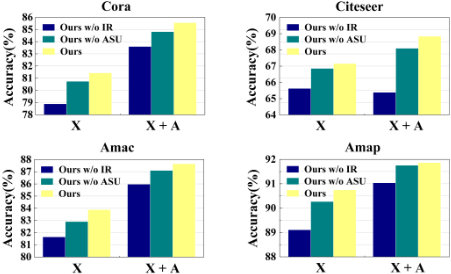
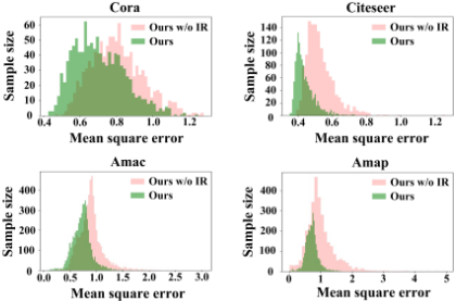
Effect of Each Component. To verify the benefit of each component, we conduct ablation studies on four datasets for ITR and two ITR variants, each of which has one of the key components removed. ITR w/o IR and ITR w/o ASU indicate the method with information recomposing and affinity structure updating being masked, respectively. From the results in Fig. 2, we observe that the accuracy of ITR on the four datasets would degrade without one of the key components. Specifically, for the "X" task, ITR exceeds ITR w/o IR by 2.54%, 1.53%, 2.24%, and 1.64% accuracy increment, and ITR w/o ASU by 0.69%, 0.30%, 0.98%, and 0.55% accuracy increment on Cora, Citeseer, Amac, and Amap, respectively. We find that the information recomposing scheme plays a more important role than the information refining scheme. To visually illustrate this point, we present the mean square error (MSE) comparison of ITR and ITR w/o IR at the last training iteration. As seen in Fig. 3, it is obvious that, with the information recomposing scheme, the method can achieve a good convergence as well as a high-quality attribute restoration.
Analysis of the Observed Ratio. To further show the superiority of ITR, we compare it with the strongest baseline SAT on Cora and Citeseer by varying the observed ratio from 20% to 80%. As shown in Table 5, taking the results of Recall@10
on Citeseer for example, our ITR outperforms SAT by 1.10%, 1.85%, 2.29%, and 2.63% with the variation of observed ratio from 20% to 80%. The improvement is more significant with the increase in the observed ratio. This observation has well verified the robustness of our ITR.
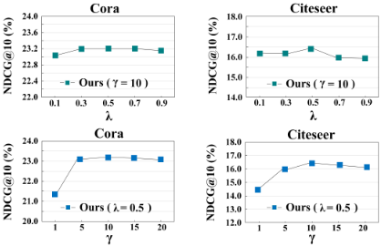
Hyper-parameter Analysis. Fig. 4 reports the NDCG@10 performance variation of ITR on Cora and Citeseer when λ and γ vary from 0.1 to 0.9 and 1 to 20, respectively. From the figures, we observe that 1) for a specific γ value, the performance shows a trend of first rising and then dropping slightly with the variation of λ. This indicates that our ITR needs a proper coefficient for auxiliary loss to rebuild the adjacency matrix. The observations of γ are similar; 2) ITR tends to perform well by setting λ and γ to 0.5 and 10, respectively.
5 Conclusion
In this work, we have designed a novel graph attribute imputation approach called ITR toward attribute-missing graph representation learning. In our method, an initializing then refining strategy is carefully designed to perform data imputation in an adaptive manner. By this means, two-source information is allowed to sufficiently negotiate with each other in the latent space. Thus the expressive capacity of imputed variables can be improved for high-quality attribute restoration. Extensive experimental results have verified the superiority and effectiveness of our proposed ITR.
Acknowledgments
This work is supported by the National Key R&D Program of China (Grant No. 2018YFB1800202, 2020YFC2003400, and 2020AAA0107100), the National Natural Science Foundation of China (Grant No. 61922088, 62006237, 62072465, 62162024, and 62162022).
@inproceedings{ijcai2022p485,
  title     = {Initializing Then Refining: A Simple Graph Attribute Imputation Network},
  author    = {Tu, Wenxuan and Zhou, Sihang and Liu, Xinwang and Liu, Yue and Cai, Zhiping and Zhu, En and Zhang, Changwang and Cheng, Jieren},
  booktitle = {Proceedings of the Thirty-First International Joint Conference on
               Artificial Intelligence, {IJCAI-22}},
  publisher = {International Joint Conferences on Artificial Intelligence Organization},
  editor    = {Luc De Raedt},
  pages     = {3494--3500},
  year      = {2022},
  month     = {7},
  note      = {Main Track},
  doi       = {10.24963/ijcai.2022/485},
  url       = {https://doi.org/10.24963/ijcai.2022/485},
}
TY - CPAPER TI - Initializing Then Refining: A Simple Graph Attribute Imputation Network AU - Tu, Wenxuan AU - Zhou, Sihang AU - Liu, Xinwang AU - Liu, Yue AU - Cai, Zhiping AU - Zhu, En AU - Zhang, Changwang AU - Cheng, Jieren T2 - Proceedings of the Thirty-First International Joint Conference on Artificial Intelligence, IJCAI-22 PB - International Joint Conferences on Artificial Intelligence Organization PY - 2022 SP - 3494 EP - 3500 DO - 10.24963/ijcai.2022/485 UR - https://doi.org/10.24963/ijcai.2022/485 ER -Copied
Machine-readable versions of this paper, for tools and AI agents:





