
Multi-Task Personalized Learning with Sparse Network Lasso
Proceedings of the Thirty-First International Joint Conference on Artificial Intelligence. Main Track. Pages 3516-3522.
https://doi.org/10.24963/ijcai.2022/488
Keywords
- Machine Learning: Multi-task and Transfer Learning
- Machine Learning: Learning Sparse Models
- Machine Learning: Regression
- Humans and AI: Personalization and User Modeling
Abstract
Multi-task learning learns multiple related tasks together, in order to improve the generalization performance. Existing methods typically build a global model shared by all the samples, which saves the homogeneity but ignores the individuality (heterogeneity) of samples. Personalized learning is recently proposed to learn sample-specific local models by utilizing sample heterogeneity, however, directly applying it in the multi-task learning setting poses three key challenges: 1) model sample homogeneity, 2) prevent from over-parameterization and 3) capture task correlations. In this paper, we propose a novel multi-task personalized learning method to handle these challenges. For 1), each model is decomposed into a sum of global and local components, that saves sample homogeneity and sample heterogeneity, respectively. For 2), regularized by sparse network Lasso, the joint models are embedded into a low-dimensional subspace and exhibit sparse group structures, leading to a significantly reduced number of effective parameters. For 3), the subspace is further separated into two parts, so as to save both commonality and specificity of tasks. We develop an alternating algorithm to solve the proposed optimization problem, and extensive experiments on various synthetic and real-world datasets demonstrate its robustness and effectiveness.
- [Barzilai and Crammer, 2015] Aviad Barzilai and Koby Crammer. Convex multi-task learning by clustering. In Artificial Intelligence and Statistics, pages 65-73. PMLR, 2015.
- [Black and Rangarajan, 1996] Michael J Black and Anand Rangarajan. On the unification of line processes, outlier rejection, and robust statistics with applications in early vi- sion. International journal of computer vision, 19(1):57- 91, 1996.
- [Chang et al., 2021] Wei Chang, Feiping Nie, Rong Wang, and Xuelong Li. New tight relaxations of rank minimiza- tion for multi-task learning. In Proceedings of the 30th ACM International Conference on Information & Knowl- edge Management, pages 2910-2914, 2021.
- [Chen et al., 2009] Jianhui Chen, Lei Tang, Jun Liu, and Jieping Ye. A convex formulation for learning shared structures from multiple tasks. In Proceedings of the 26th Annual International Conference on Machine Learning, pages 137-144, 2009.
- [Gong et al., 2012] Pinghua Gong, Jieping Ye, and Chang- shui Zhang. Robust multi-task feature learning. In Pro- ceedings of the 18th ACM SIGKDD international con- ference on Knowledge discovery and data mining, pages 895-903, 2012.
- [Gong et al., 2013] Pinghua Gong, Jieping Ye, and Chang- shui Zhang. Multi-stage multi-task feature learning. The Journal of Machine Learning Research, 14(1):2979-3010, 2013.
- [Hallac et al., 2015] David Hallac, Jure Leskovec, and Stephen Boyd. Network lasso: Clustering and optimiza- tion in large graphs. In Proceedings of the 21th ACM SIGKDD international conference on knowledge discov- ery and data mining, pages 387-396, 2015.
- [Han and Zhang, 2015] Lei Han and Yu Zhang. Learning multi-level task groups in multi-task learning. In Twenty- Ninth AAAI Conference on Artificial Intelligence, 2015.
- [Han and Zhang, 2016] Lei Han and Yu Zhang. Multi-stage multi-task learning with reduced rank. In Proceedings of the AAAI Conference on Artificial Intelligence, volume 30, 2016.
- [Jeong and Jun, 2018] Jun-Yong Jeong and Chi-Hyuck Jun. Variable selection and task grouping for multi-task learn- ing. In Proceedings of the 24th ACM SIGKDD Interna- tional Conference on Knowledge Discovery & Data Min- ing, pages 1589-1598, 2018.
- [Kumar and Daumé, 2012] Abhishek Kumar and Hal Daumé. Learning task grouping and overlap in multi-task learning. In Proceedings of the 29th International Cofer- ence on International Conference on Machine Learning, ICML'12, page 1723-1730, Madison, WI, USA, 2012. Omnipress.
- [Lee et al., 2010] Seunghak Lee, Jun Zhu, and Eric P. Xing. Adaptive multi-task lasso: with application to eqtl detec- tion. In NIPS, pages 1306-1314.
- Curran Associates, Inc., 2010.
- [Lengerich et al., 2018] Benjamin J Lengerich, Bryon Aragam, and Eric P Xing. Personalized regression enables sample-specific pan-cancer analysis. Bioinformatics, 34(13):i178-i186, 2018.
- [Li et al., 2018] Jundong Li, Liang Wu, Harsh Dani, and Huan Liu. Unsupervised personalized feature selection. In Proceedings of the AAAI Conference on Artificial Intel- ligence, volume 32, 2018.
- [Nesterov, 2013] Y Nesterov. Introductory Lectures on Con- vex Optimization: A Basic Course, volume 87. Springer Science & Business Media, 2013.
- [Okazaki and Kawano, 2021] Akira Okazaki and Shuichi Kawano. Multi-task learning for compositional data via sparse network lasso. arXiv preprint arXiv:2111.06617, 2021.
- [Petrovich and Yamada, 2020] Mathis Petrovich and Makoto Yamada. Fast local linear regression with anchor regular- ization. arXiv preprint arXiv:2003.05747, 2020.
- [Pong et al., 2010] Ting Kei Pong, Paul Tseng, Shuiwang Ji, and Jieping Ye. Trace norm regularization: Reformula- tions, algorithms, and multi-task learning. SIAM Journal on Optimization, 20(6):3465-3489, 2010.
- [Tibshirani, 1996] Robert Tibshirani. Regression shrinkage and selection via the lasso. Journal of the Royal Statistical Society: Series B (Methodological), 58(1):267-288, 1996.
- [Xu et al., 2015] Jianpeng Xu, Jiayu Zhou, and Pang-Ning Tan. Formula: Factorized multi-task learning for task dis- covery in personalized medical models. In Proceedings of the 2015 SIAM International Conference on Data Mining, pages 496-504. SIAM, 2015.
- [Yamada et al., 2017] Makoto Yamada, Takeuchi Koh, To- moharu Iwata, John Shawe-Taylor, and Samuel Kaski. Lo- calized lasso for high-dimensional regression. In Artificial Intelligence and Statistics, pages 325-333. PMLR, 2017.
- [Yang et al., 2019] Zhiyong Yang, Qianqian Xu, Yang- bangyan Jiang, Xiaochun Cao, and Qingming Huang. Generalized block-diagonal structure pursuit: Learning soft latent task assignment against negative transfer. In H. Wallach, H. Larochelle, A. Beygelzimer, F. d'Alché- Buc, E. Fox, and R. Garnett, editors, Advances in Neural Information Processing Systems, volume 32.
- [Zhang and Yang, 2021] Yu Zhang and Qiang Yang. A sur- vey on multi-task learning. IEEE Transactions on Knowl- edge and Data Engineering, pages 1-1, 2021.
References were extracted automatically from the PDF and may contain errors.
Full text extracted automatically from the PDF; figures, tables and equations may differ. The PDF is the version of record.
1 Introduction
Multi-Task Learning (MTL) is an emerging machine learning topic, which seeks to improve the generalization performance of multiple learning tasks by sharing common information across them. It has been applied in many real-world applications, such as computer vision, natural language processing, bioinformatics analysis and ubiquitous computing [Zhang and Yang, 2021]. The key challenge in MTL is how to capture task correlations among different tasks. To tackle this challenge, various methods have been proposed in the MTL literature. Feature learning approach [Lee et al., 2010; Gong et al., 2013] and low-rank approach [Chen et al., 2009; Pong et al., 2010] assume that all the tasks are correlated by sharing common low-dimensional subspace. Task clustering approach [Kumar and Daum´e, 2012; Barzilai and Crammer, 2015] expects to learn the group structure among tasks. Decomposition approach [Gong et al., 2012; Han and Zhang, 2015] assumes that two or more components of models can be combined for robust prediction. Despite much success they have achieved, these MTL methods save only sample homogeneity by learning one common global model shared by samples of each task, and thus ignore the individuality (heterogeneity) of samples.
Taking into account the heterogeneity of different samples, Personalized Learning (PL) is proposed, which allows each sample to have its own prediction model. For example, in disease prediction, the heterogeneity of patients enables them to have their own predictive models. The major challenge of PL is how to prevent from overfitting by limiting the number of effective parameters of personalized models. To handle this challenge, several methods have been proposed, based on the network Lasso [Hallac et al., 2015; Yamada et al., 2017], matrix factorization [Xu et al., 2015], anchor regularization [Petrovich and Yamada, 2020], and distance-matching [Lengerich et al., 2018].
Experimental results in a variety of applications have shown the performance superiority of MTL and PL against baseline learners. However, no MTL method has considered sample heterogeneity, and directly applying PL in the MTL scenarios may suffer from three main problems. 1) PL methods usually ignore sample homogeneity, and the ignorance of either heterogeneity or homogeneity of samples probably harms the generalization performance. 2) Building samplespecific local models needs to learn a potentially large number of parameters, making it prone to overfitting, and this problem becomes severer when learning multiple tasks together. 3) Capturing task correlations is crucial for performance improvement inMTL, but it is difficult for existing PL methods to do so.
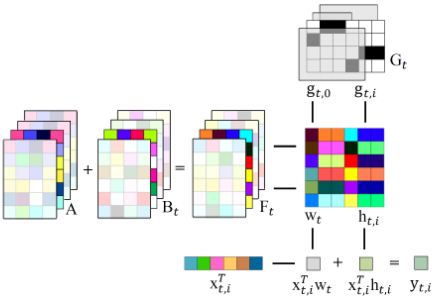
To address the aforementioned problems, in this paper, we propose a novel Multi-Task Personalized Learning (MTPL) method. Specifically, the personalized model in MTPL is decomposed into a sum of global and local models, in order to save both homogeneity and heterogeneity of samples (for Problem 1). To reduce the effective number of parameters (for Problem 2), the joint models are projected into a low-dimensional subspace, in which local models of similar samples exhibit a common group structure via sparse network Lasso. Moreover, the subspace is separated into one task-common part and one task-specific part, aiming to capture task correlations and task specificity, respectively (for Problem 3). We illustrate the framework of MTPL in Fig. 1. We develop an alternating algorithm to solve the proposed optimization problem. Empirical results on both synthetic and real-world datasets demonstrate the superiority of MTPL. The contributions of this work can be summarized as follows:
- We propose a novel method, named MTPL, to explicitly save both sample homogeneity and sample heterogeneity in the MTL scenarios.
- To avoid overfitting, we propose to use sparse network lasso to regularize low-rank matrix factorization and promote a sparse group structure of local models.
- We develop an alternating algorithm to solve the optimization problem of MTPL, and show its effectiveness on both synthetic and real-world datasets.
2 RelatedWorks
Multi-task learning (MTL) expects to improve the performance of multiple prediction tasks by sharing common knowledge across them. One way to capture task relationship is to constrain the model parameter matrix to be low rank. Low-rank matrix factorization [Chen et al., 2009] or the trace norm based regularization [Pong et al., 2010] can be applied to achieve this goal. RAMUSA [Han and Zhang, 2016] introduces the capped trace norm that punishes only the singular values smaller than a given threshold. KMSV [Chang et al., 2021] uses a new tight relaxation of rank minimization based on two kinds of regularizations. Recent studies have focused on learning group structures among tasks [Kumar and Daum´e, 2012; Barzilai and Crammer, 2015]. VSTGMTL [Jeong and Jun, 2018] performs variable selection and learns an overlapping group structure among tasks. [Yang et al., 2019] proposes to learn the grouping structure based on the block-diagonal task assignment matrix.
Personalized learning (PL) allows each sample to have its sample-specific local model. The network Lasso [Hallac et al., 2015] estimates personalized models by simultaneously clustering and optimizing the parameters in graphs. The localized Lasso [Yamada et al., 2017] learns sparse local models by incorporating a sample-wise exclusive group regularizer with the network Lasso. [Okazaki and Kawano, 2021] proposes a personalized learning method specific for compositional data, based on the sparse network Lasso and the symmetric form of the log-contrast model. UPFS [Li et al., 2018] performs personalized feature selection by finding shared features for all instances and discriminative features specific for each instance at the same time. FORMULA [Xu et al., 2015] treats the personalized model of each sample as a task, and transforms it to a MTL problem, that is solved by low-rank decomposition. [Lengerich et al., 2018] proposes a distancematching regularization with covariates as extra input, that regularizes the model parameters based on the assumption that similar parameters share similar covariates. [Petrovich and Yamada, 2020] proposes the FALL model, in which the separated models are regularized to be similar to the precomputed anchor models in a two-stage manner.
Previous MTL methods mainly focus on learning multiple global models together under the assumption of sample homogeneity, which significantly limits their applications on real-world problems where data exhibits strong sample heterogeneity. PL enables to cope with the heterogeneity, but in the MTL scenarios, it faces the challenges of avoiding overparameterization and exploiting task correlations. In contrast, the proposed MTPL not only captures the correlations among multiple tasks, but also saves both heterogeneity and homogeneity of samples in an efficient way, leading to a significantly reduced number of effective parameters and thus avoiding overfitting.
3 The ProposedMethod
3.1 Preliminary
Given m tasks, the t-th task is associated with the training data (Xt, yt), t = 1, 2, ...,m, that lies in the d-dimensional feature space. The i-th row of the data matrix Xt ∈ Rnt×d is denoted by xt,i ∈ Rd , corresponding to the i-th sample in the t-th task, and the i-th entry of the target vector yt ∈ Rnt is denoted by yt,i ∈ R, where nt is the number of samples in the t-th task. Without loss of generality, for an arbitrary matrix A, ‖A‖F and ‖A‖1 denote the Frobenius norm and the ℓ1norm, respectively. Additionally, we define the ℓ2-norm of an arbitrary vector a as ‖a‖2.
To apply PL in the MTL setting, a simple and straightforward way is to learn the following personalized model,
where θt,i ∈ Rd denotes the regression coefficients for the ith sample xt,i. We consider linear models in this paper, and it can be easily extended to non-linear cases by kernel methods. For simplicity, the intercept is omitted in (1) by assuming the input data has been centered in column-wise.
3.2 Methodology
The personalized model in (1) captures the individually (heterogeneity) of samples, and it ignores sample homogeneity, i.e., similar samples in one task may have something in common. For example, in score prediction, although the predictive model for each student varies a lot, students in the same school share some common characteristics, such as reference books and school denomination. Therefore, it is important to leverage the homogeneity by capturing globally shared features. To this end, we propose to decompose the personalized model θt,i into a sum of a global model wt and a local model ht,i, yielding the reformulation of (1):
where wt helps to save important features shared by all samples in task t, and ht,i identifies useful features specific for sample i. In other words, the personalized model in (2) enables to save both homogeneity and heterogeneity of samples.
Building the personalized models in (2) for all samples is computationally expensive, and the large number of parameters in wt and ht,i (∀t, i) makes it vulnerable to overfitting. To address this problem, we assume that samples belong to the same task are correlated through a subspace constructed by a limited number of latent bases. Therefore, instead of directly learning wt and ht,i (∀t, i), we impose a low-rank constraint on them by applying matrix factorization:
where Ft ∈ Rd×K (K ≪ d, nt) with each column corresponding to one latent basis, gt,0 and gt,i ∈ RK are the loading assignments of the global model wt and the local model ht,i, respectively. The low-rank matrix factorization not only saves sample correlations but also controls overfitting by reducing the model size. In addition, to further reduce the number of parameters, we consider that similar local loading assignments {gt,i}nt i=1 can be grouped together based on an identical parameter subset, that makes each local model is reconstructed by only a few latent bases. To this end, inspired by the network Lasso [Hallac et al., 2015], we impose the sparse network Lasso on the loading assignments:
where Gt = [gt,0, gt,1, ..., gt,nt ] ∈ RK×(nt+1) is the joint assignment matrix, λ is a positive hyper-parameter, and stij measures the similarity between xt,i and xt,j according to:
In (5), σ is a given constant, and Nk(xt,i) is the set of knearest neighbors of xt,i. In (4), the ℓ2-norm penalty, instead of the squared ℓ2-norm penalty, is imposed on the difference between local assignments gt,i and gt,j, incentivizing the difference to be exactly zero, rather than just close to zero. It promotes similar assignments to be grouped together and share the same parameters. Besides, the ℓ1-norm penalty on Gt encourages sparsity among the assignments within a specific group. In this way, sparse network Lasso encourages a sparse group structure among {gt,i}, that saves sample correlations and further reduces the model size. In [Okazaki and Kawano, 2021], the sparse network Lasso is directly imposed on the local model, resulting in a high possibility of shrinking the coefficients of some samples towards zero. In contrast, (4) avoids such a risk by imposing the sparse network Lasso on the joint model, which gives another chance for θt,i = wt + ht,i ̸= 0, even if the local model ht,i = 0.
The aforementioned formulation is developed in the single task setting and ignores task correlations. In the MTL scenarios, modeling correlations among tasks is crucial to improve the generalization ability. Hence, we expect that the t-th latent basis matrix Ft can be represented as a combination of a task-common part and a task-specific part, i.e.,
where A contains the task-common latent bases, while Bt is the task-specific latent basis matrix that stores the specificity of the t-th task. Therefore, correlations among tasks are captured without sacrificing the specificity of individual tasks.
By combining (2), (3), (4) and (6), the optimization problem of the proposed MTPL method is defined by
where λ1, λ2 and λ3 are positive hyper-parameters. The Frobenius norm based regularizations of A and Bt controls the complexity of the personalized models. Thus, the proposed MTPL in (7) successfully builds personalized models by taking into account homogeneity and heterogeneity among samples in an efficient manner, and captures both task commonality and task specificity in the MTL scenarios.
3.3 Prediction
To make the prediction on an unseen testing sample ˆxt in the t-th task, we can solve the following Weber problem [Hallac et al., 2015] to learn its personalized model ˆθt:
where k is the number of neighbors of ˆxt in the training data {xt,i}nt i=1 , and sti measures the similarity between ˆxt and its neighbor xt,i. The above problem can be efficiently solved by an iterative algorithm, and the details are provided in the supplement 1 . Finally, we obtain the prediction by ˆ yt = ˆxTt ˆθt.
4 Optimization Algorithm
The optimization problem in (7) is not jointly convex, but it is convex w.r.t. A, Bt and Gt, respectively. Hence, we propose to solve it by an alternating optimization algorithm. Before presenting the update procedures, we reformulate the loss function in (7) by:
1 We provide the supplementary material of MTPL at: https:// github.com/JiankunWang912/MTPL.
where Xt ∈ Rnt×dnt is block diagonal matrix with the ith block being xTt,i , i = 1, 2, ..., nt, Mt = [1Tnt ; Int ] ∈ R(nt+1)×nt with 1nt being the all-one vector in size of nt, and vec(·) denotes the vectorization of a matrix.
4.1 Updating Gt
With fixed A and Bt, the problem w.r.t. Gt becomes:
Based on the Black-Rangarajan Duality [Black and Rangarajan, 1996], we introduce an auxiliary variable lt i,j for the sample pair (xt,i, xt,j), and optimize an equivalent problem:
where 1 4 (lt i,j )-1 is a penalty on ignoring the connection between xt,i and xt,j. The derivation of (11) can be found in the supplementary material.
When Gt is fixed, we obtain the closed-form solution of lt i,j by setting the derivative of (11) w.r.t. lt i,j to be zero, i.e.,
When L is fixed, we rewrite the problem in matrix form:
where Dt ∈ Rnt×nt is a diagonal matrix with the i-th diagonal element dtii = ∑nt j=1 stij lt ij (i = 1, ..., nt), Wt ∈ Rnt×nt is a symmetric matrix with wt ij = stij lt ij (i, j = 1, ..., nt), Nt = [0Tnt ; Int ] ∈ R(nt+1)×nt is an auxiliary matrix, and tr(·) is the trace of a matrix. Then, proximal gradient descent method [Nesterov, 2013] can be applied to update Gt. The gradient of the objective in (13) w.r.t. vec(Gt) is given by:
where Pt = Xt(MTt ⊗ (A+Bt)), and ⊗ is the Kronecker product. The derivation of (14) is given in the supplement. Then, the update rule is:
where ∇f(Gt) is obtained by reshaping ∇f(vec(Gt)), µ is the learning rate and soft(a, b) = sign(a)max(|a| - b, 0) is the soft thresholding operator.
4.2 Updating Bt
With fixed A and Gt, the objective function w.r.t. Bt becomes:
By setting the derivative of L(Bt) w.r.t. vec(Bt) to be zero, we obtain the closed-form solution:
4.3 Updating A
When {Bt}mt=1 and {Gt}mt=1 are fixed, the objective function w.r.t. A is reformulated as:
Similarly, we obtain the closed-from solution:
5 Experiments
5.1 Experimental Setting
Synthetic Data
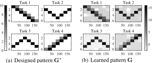
To generate synthetic datasets, we set the number of tasks as m = 4, and assume that each task has the same number (n = 175) of samples. The dimensionality d of each sample is set as 20, and the dimensionality of the latent subspace is set as K = 6. Entries of A ∈ Rd×K and Bt ∈ Rd×K are sampled from normal distributions N(0, 1) and N(0, 4), respectively. We set gt,0, the global loading assignment in task t, to be a K-dimensional vector with the t-th entry being 1 and the rest being 0 (m < K). The i-th local loading assignment gt,i is specially defined with a sparse pattern, as illustrated in Fig. 2(a), and every 25 samples in a task lie in the same cluster and thus share the same sparse pattern. The similarity matrix S is designed as a block diagonal matrix with the main-diagonal blocks being matrices of all ones. The ground truth personalized model is calculated by θt,i = (A+Bt)(gt,0 + gt,i), t = 1, ...,m, i = 1, ..., n. Finally, the target is calculated by yt,i = xTt,iθt,i + δt,i, where xt,i is randomly sampled from a normal distribution N(0, 1), and δt,i is zero-mean Gaussian noise following N(0, 0.01).
Real-World Data
We conduct experiments on six real-world multi-task datasets: School 2 , SARCOS 3 , Sales 4 , Parkinsons 4 , Computer 5 and Isolet 6 . Table 1 summarizes their statistics. Details of the datasets are provided in the supplement.
2 https://github.com/jiayuzhou/MALSAR/tree/master/data
3 http://www.gaussianprocess.org/gpml/data
4 https://archive.ics.uci.edu/ml/datasets.php
5 https://github.com/probml/pmtk3/tree/master/data
6 http://www.cad.zju.edu.cn/home/dengcai/Data/MLData.html
| Datasets | #Samples | #Features | #Tasks |
|---|---|---|---|
| School | 15362 | 27 | 139 |
| SARCOS | 48933 | 21 | 7 |
| Sales | 38117 | 5 | 811 |
| Parkinsons | 5875 | 16 | 42 |
| Computer | 20 | 13 | 190 |
| Isolet | 7797 | 617 | 5 |
Comparing Methods
We compare MTPL 7 with two types of learning methods, single-task PL and MTL. For single-task PL, we compare MTPL with FORMULA [Xu et al., 2015], Network Lasso [Hallac et al., 2015] and Localized Lasso [Yamada et al., 2017]. FORMULA regards each instance as a task and adopts a multi-task type method, and Localized Lasso is a sparse variant of Network Lasso, which groups local models in graphs. For MTL, we compare MTPL with three state-of-the-art methods: VSTG [Jeong and Jun, 2018], GBDSP [Yang et al., 2019] and KMSV [Chang et al., 2021]. VSTG and GBDSP are proposed based on the assumption that tasks have a latent group structure, and KMSV is developed by a new low-rank approach. Lasso [Tibshirani, 1996] is selected as the baseline method, which learns a sparse prediction model for each task independently.
Configuration
For evaluation, we randomly select 60%, 20% and 20% of total samples for training, testing and validation, respectively. We repeat this process by ten times, and report the mean with standard deviation in terms of three metrics: root mean squared error (RMSE), normalized mean squared error (NMSE) and mean absolute error (MAE). The number K of latent bases in GBDSP, VSTG, FORMULA and MTPL is selected from {3, 5, 7, 9, 11}. The value k of similarity function used in Network Lasso, Localized Lasso and MTPL is fixed to be 5. The value k of k-support norm in VSTG is selected from {1, 2, 3}. The number of transfer groups in GBDSP is selected from {3, 5, 7, 9, 11}. The search grid for the other hyper-parameters is set as {2-10 , 2-8 , · · · , 28 , 210 }. For each iterative algorithm, we terminate it once the relative change of its objective is below 10-5 , and set the maximum number of iterations as 1000.
5.2 Experiments on Synthetic Data
Illustration of Structured Sparsity
We illustrate the recovery of sparsity patterns w.r.t. the factor loading matrix on the designed synthetic dataset in Fig. 2, where G∗ denotes the designed factor loading matrix, and G is the matrix learned by MTPL with the setting λ1 = 22 , λ2 = 28 and λ3 = 26 . As shown is Fig. 2, MTPL successfully recovers the structured sparsity pattern in each task. This demonstrates the effectiveness of sparse network Lasso used in MTPL, which jointly performs sample grouping and feature selection.
7 We provide the MATLAB code of MTPL at: https://github.com/ JiankunWang912/MTPL.
Analysis on Sample Correlation Modeling
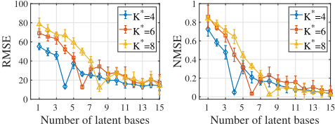
In order to model sample correlations, MTPL assumes that personalized models in a task are constructed based on a limited number K of latent bases. It reduces the number of effective parameters and avoids overfitting. To evaluate this effect, we generate three synthetic datasets with different ground truth K∗ ∈ {4, 6, 8}, and apply MTPL on each dataset with the value of K varying from 1 to 15 by step 1. Fig. 3 shows the experiment results of MTPL in RMSE and NMSE. As shown in Fig. 3, as the value of K increases, the performance rises first, and then stabilizes. Note that MTPL always achieves the best performance when K = K∗ . Therefore, MTPL has a chance to reduce computational complexity without compromising prediction accuracy, once samples are indeed constructed by a small number of latent bases.
5.3 Experiments on Real-World Data
Evaluation of Comparing Methods
To evaluate the comparing methods, we conduct an experiment on six multi-task datasets, and report the results in RMSE, NMSE and MAE by Table 2, where the best performance is highlighted in boldface. From Table 2, we can see that MTPL obtains the best performance in 12 cases out of total 18 cases. This performance superiority probably originates from two perspectives. First, MTPL decomposes each personalized model into a sum of global and local models, enabling to save both heterogeneity and homogeneity of samples. Second, MTPL promotes structured sparsity via sparse network Lasso, which reduces the number of effective parameters, and avoids overfitting. MTL methods outperform STL methods on most of the datasets. However, on the Isolet dataset, two single-task PL methods, Network Lasso and Localized Lasso, perform better than MTL methods except MTPL, probably due to the high heterogeneity of samples in Isolet. In terms of MTL methods, VSTG and GBDSP outperform KMSV, indicating the importance on capturing group structures among tasks.
| Dataset | Metric | LASSO | FORMULA | Network Lasso | Localized Lasso | VSTG | GBDSP | KMSV | MTPL |
|---|---|---|---|---|---|---|---|---|---|
| School | RMSE NMSE MAE | 10.3003(0.0309) 0.8452(0.0212) 8.2801(0.0222) | 10.2341(0.0095) 0.7937(0.0003) 8.2515(0.0102) | 10.2335(0.0096) 0.7906(0.0004) 8.2393(0.0091) | 10.2397(0.0097) 0.7892(0.0003) 8.2376(0.0087) | 9.8671(0.0147) 0.8229(0.0726) 8.6501(2.3316) | 9.8934(0.0145) 0.7404(0.0002) 7.9329(0.0093) | 10.0654(0.0087) 0.7686(0.0004) 8.0577(0.0089) | 9.8220(0.0115) 0.7300(0.0002) 7.8759(0.0071) |
| SARCOS | RMSE NMSE MAE | 2.8083(0.0161) 0.1324(0.0001) 2.0661(0.0049) | 3.5471(0.0253) 0.3134(0.0003) 2.6348(0.0138) | 3.2515(0.0313) 0.1061(0.0000) 2.1355(0.0046) | 4.1375(0.0380) 0.1849(0.0001) 2.8239(0.0118) | 2.6585(0.0091) 0.1247(0.0001) 1.9267(0.0035) | 2.6633(0.0095) 0.1256(0.0001) 1.9276(0.0037) | 2.9049(0.0090) 0.3793(0.0103) 2.1474(0.0052) | 1.9830(0.0048) 0.0669(0.0001) 1.3921(0.0019) |
| Sales | RMSE NMSE MAE | 0.2311(0.0000) 1.0706(0.0001) 0.1877(0.0000) | 0.2340(0.0000) 1.1136(0.0001) 0.1912(0.0000) | 0.2301(0.0000) 1.0683(0.0001) 0.1866(0.0000) | 0.2290(0.0000) 1.0553(0.0000) 0.1863(0.0000) | 0.2274(0.0000) 1.1216(0.0657) 0.1968(0.0005) | 0.2269(0.0000) 1.0433(0.0003) 0.1850(0.0000) | 0.2283(0.0000) 1.0563(0.0000) 0.1871(0.0000) | 0.2268(0.0000) 1.0433(0.0000) 0.1852(0.0000) |
| Isolet | RMSE NMSE MAE | 4.9374(0.0070) 0.4355(0.0002) 3.9071(0.0050) | 4.5400(0.2733) 0.3774(0.0098) 3.0556(0.2560) | 3.5111(0.0120) 0.2232(0.0002) 2.1576(0.0045) | 3.6708(0.0169) 0.2421(0.0003) 2.0905(0.0065) | 4.9257(0.0109) 0.4334(0.0003) 3.8976(0.0063) | 4.9077(0.0094) 0.4303(0.0003) 3.8868(0.0062) | 5.7518(0.0065) 0.5903(0.0002) 4.6824(0.0074) | 3.5995(0.0041) 0.2329(0.0000) 2.3023(0.0030) |
| Parkinsons | RMSE NMSE MAE | 2.2651(0.0627) 1.6729(0.6741) 1.7768(0.0125) | 2.1400(0.0015) 1.4387(0.0330) 1.7393(0.0009) | 2.1160(0.0405) 1.2169(0.1346) 1.6287(0.0029) | 1.9628(0.0018) 0.9713(0.0013) 1.6018(0.0007) | 1.9658(0.0099) 1.0051(0.0215) 1.6191(0.0023) | 2.0156(0.0250) 1.0824(0.0500) 1.6175(0.0015) | 1.9834(0.0083) 1.0207(0.0061) 1.6280(0.0019) | 1.9421(0.0077) 0.9738(0.0079) 1.5842(0.0005) |
| Computer | RMSE NMSE MAE | 1.7794(0.0041) 1.7393(0.0224) 1.5200(0.0027) | 2.2835(0.0059) 2.4711(0.3172) 1.9435(0.0049) | 2.5175(0.0049) 4.3934(0.1876) 2.1859(0.0048) | 1.7983(0.0041) 1.6715(0.0374) 1.5404(0.0022) | 1.6348(0.0034) 1.5426(0.0451) 1.4096(0.0024) | 1.6851(0.0032) 1.6020(0.0669) 1.4435(0.0027) | 1.7283(0.0056) 1.7152(0.1043) 1.4853(0.0042) | 1.6409(0.0042) 1.5379(0.0227) 1.4010(0.0031) |
Analysis on the Effect of Model Decomposition
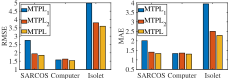
To evaluate the effect of model decomposition θt,i = wt + ht,i used in MTPL, an experiment is performed by comparing MTPL with two special variants: the gobal MTPL1 (θ(1) t,i = wt) and the local MTPL2 (θ(2) t,i = ht,i). Evaluation results on the SARCOS, Computer and Isolet datasets are shown in Fig. 4. The results for the other three datasets are similar. From Fig. 4, we can see that MTPL and MTPL2 outperform MTPL1 on the SARCOS and Isolet datasets, while MTPL and MTPL1 perform better than MTPL2 on the Computer dataset. The superior performance of MTPL in all cases shows that it is important to save both heterogeneity and homogeneity of samples by model decomposition.
Hyperparameter Sensitivity Analysis
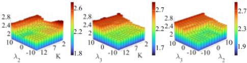
The sensitivity 8 of MTPL in three hyper-parameters λ2, λ3 and K is investigated on the SARCOS dataset. Specifically, λ2 controls the structured sparsity among local models, λ3 controls the sparsity of Gt and K is the dimension of shared latent subspace. The parameters λ2, λ3 are selected from {2-10 , 2-8 , · · · , 28 , 210 }, while the value ofK is varied from 2 to 12 by step 1. Three experiments are conducted to evaluate the pairwise correlations. The first experiment on λ2 and K is conducted by fixing λ1 = λ3 = 1, and similar setting is applied for the other two experiments. Fig. 5 show the results in RMSE. As shown in Fig. 5, we can conclude that: (1) as the value of K increases, the performance first rises and then keeps steady once K ≥ 7; (2) the best performance on SARCOS is achieved by setting λ2 ≤ 24 and λ3 ≤ 20 .
6 Conclusion
We proposed a novel method, MTPL, to apply personalized learning in multi-task scenarios. MTPL enables to save homogeneity and heterogeneity of samples by the global model and the local model, respectively. Thanks to sparse network lasso, it promotes sparse group structures of local models in the latent subspace found by low-rank matrix factorization, which reduces the model size and avoids overfitting. To tackle the challenge of MTL, MTPL captures both task commonality and task specificity via matrix decomposition. We developed an alternating algorithm to optimize the proposed objective function. Experiments indicate that MTPL is effective for a wide range of multi-task applications.
8 The analysis on λ1 is not shown here, as it is insensitive to the value change, and we recommend to set it by λ1 ≤ 26 .
@inproceedings{ijcai2022p488,
  title     = {Multi-Task Personalized Learning with Sparse Network Lasso},
  author    = {Wang, Jiankun and Sun, Lu},
  booktitle = {Proceedings of the Thirty-First International Joint Conference on
               Artificial Intelligence, {IJCAI-22}},
  publisher = {International Joint Conferences on Artificial Intelligence Organization},
  editor    = {Luc De Raedt},
  pages     = {3516--3522},
  year      = {2022},
  month     = {7},
  note      = {Main Track},
  doi       = {10.24963/ijcai.2022/488},
  url       = {https://doi.org/10.24963/ijcai.2022/488},
}
TY - CPAPER TI - Multi-Task Personalized Learning with Sparse Network Lasso AU - Wang, Jiankun AU - Sun, Lu T2 - Proceedings of the Thirty-First International Joint Conference on Artificial Intelligence, IJCAI-22 PB - International Joint Conferences on Artificial Intelligence Organization PY - 2022 SP - 3516 EP - 3522 DO - 10.24963/ijcai.2022/488 UR - https://doi.org/10.24963/ijcai.2022/488 ER -Copied
Machine-readable versions of this paper, for tools and AI agents:





