
Modeling Spatio-temporal Neighbourhood for Personalized Point-of-interest Recommendation
Proceedings of the Thirty-First International Joint Conference on Artificial Intelligence. Main Track. Pages 3530-3536.
https://doi.org/10.24963/ijcai.2022/490
Keywords
- Data Mining: Knowledge Graphs and Knowledge Base Completion
- Machine Learning: Recommender Systems
Abstract
Point-of-interest (POI) recommendations can help users explore attractive locations, which is playing an important role in location-based social networks (LBSNs). In POI recommendations, the results are largely impacted by users' preferences. However, the existing POI methods model user and location almost separately, which cannot capture users' personal and dynamic preferences to location. In addition, they also ignore users' acceptance to distance/time of location. To overcome the limitations of the existing methods, we first introduce Knowledge Graph with temporal information (known as TKG) into POI recommendation, including both user and location with timestamps. Then, based on TKG, we propose a Spatial-Temporal Graph Convolutional Attention Network (STGCAN), a novel network that learns users' preferences on TKG by dynamically capturing the spatial-temporal neighbourhoods. Specifically, in STGCAN, we construct receptive fields on TKG to aggregate neighbourhoods of user and location respectively at each timestamp. And we measure the spatial-temporal interval as users' acceptance to distance/time with self-attention. Experiments on three real-world datasets demonstrate that the proposed model outperforms the state-of-the-art POI recommendation approaches.
- [Cheng et al., 2013] Chen Cheng, Haiqin Yang, Michael R. Lyu, and Irwin King. Where you like to go next: Suc- cessive point-of-interest recommendation. In IJCAI, page 2605-2611, 2013. IJCAI
- [Cho et al., 2011] Eunjoon Cho, Seth A. Myers, and Jure Leskovec. Friendship and mobility: User movement in location-based social networks. In SIGKDD, page 1082-1090, 2011.
- [Chung et al., 2014] Junyoung Chung, C ¸aglar Gülc ¸ehre, Kyunghyun Cho, and Yoshua Bengio. Empirical evalua- tion of gated recurrent neural networks on sequence mod- eling. CoRR, abs/1412.3555, 2014.
- [Feng et al., 2015] Shanshan Feng, Xutao Li, Yifeng Zeng, Gao Cong, Yeow Meng Chee, and Quan Yuan. Person- alized ranking metric embedding for next new poi recom- mendation. In ICOAI, page 2069-2075, 2015. IJCAI
- [Graves, 2008] Alex Graves. Supervised sequence labelling with recurrent neural networks. Studies in Computational Intelligence, 2008.
- [Hochreiter and Schmidhuber, 1997] Sepp Hochreiter and Jürgen Schmidhuber. Long Short-Term Memory. Neural Computation, 9(8):1735-1780, 11 1997.
- [Kang and McAuley, 2018] Wang-Cheng Kang and Julian McAuley. Self-attentive sequential recommendation. In Proceedings of the ACM IEEE International Conference on Data Mining, pages 197-206, 2018.
- [Li et al., 2020] Jiacheng Li, Yujie Wang, and Julian McAuley. Time interval aware self-attention for sequen- tial recommendation. In WSDM, page 322-330, 2020.
- [Lian et al., 2020] Defu Lian, Yongji Wu, Yong Ge, Xing Xie, and Enhong Chen. Geography-aware sequential lo- cation recommendation. In SIGKDD, page 2009-2019, 2020.
- [Liu et al., 2016] Qiang Liu, Shu Wu, Liang Wang, and Tieniu Tan. Predicting the next location: A recurrent model with spatial and temporal contexts. In AAAI, page 194-200, 2016.
- [Luo et al., 2021] Yingtao Luo, Qiang Liu, and Zhaocheng Liu. Stan: Spatio-temporal attention network for next lo- cation recommendation. In WWW, page 2177-2185, 2021.
- [Rendle et al., 2009] Steffen Rendle, Christoph Freuden- thaler, Zeno Gantner, and Lars Schmidt-Thieme. Bpr: Bayesian personalized ranking from implicit feedback. In UAI, page 452-461, 2009.
- [Schlichtkrull et al., 2018] Michael Schlichtkrull, Thomas Kipf, Peter Bloem, Rianne van den Berg, Ivan Titov, and Max Welling. Modeling relational data with graph convo- lutional networks. CoRR, abs/1703.06103, 2018.
- [Schuster and Paliwal, 1997] Mike Schuster and Kuldip K. Paliwal. Bidirectional recurrent neural networks. IEEE Transactions on Signal Processing, 45(11):2673-2681, 1997.
- [Tang and Wang, 2018] Jiaxi Tang and Ke Wang. Person- alized top-n sequential recommendation via convolutional sequence embedding. In WSDM, page 565-573, 2018.
- [Vaswani et al., 2017] Ashish Vaswani, Noam Shazeer, Niki Parmar, Jakob Uszkoreit, Llion Jones, Aidan N Gomez, Ł ukasz Kaiser, and Illia Polosukhin. Attention is all you need. In NIPS, page 5998-6008, 2017.
- [Wang et al., 2018a] Hongwei Wang, Fuzheng Zhang, Jialin Wang, Miao Zhao, Wenjie Li, Xing Xie, and Minyi Guo. Ripplenet: Propagating user preferences on the knowledge graph for recommender systems. In CIKM, page 417-426, 2018.
- [Wang et al., 2018b] Shoujin Wang, Liang Hu, Longbing Cao, Xiaoshui Huang, Defu Lian, and Wei Liu. Attention- based transactional context embedding for next-item rec- ommendation. In AAAI, pages 2532-2539, 2018.
- [Wang et al., 2019a] Hongwei Wang, Miao Zhao, Xing Xie, Wenjie Li, and Minyi Guo. Knowledge graph convolu- tional networks for recommender systems. In WWW, page 3307-3313, 2019.
- [Wang et al., 2019b] Xiang Wang, Xiangnan He, Yixin Cao, Meng Liu, and Tat-Seng Chua. Kgat: Knowledge graph attention network for recommendation. In SIGKDD, page 950-958, 2019.
- [Wang et al., 2021] Shoujin Wang, Liang Hu, Yan Wang, Xi- angnan He, Quan Z Sheng, Mehmet A Orgun, Longbing Cao, Francesco Ricci, and Philip S Yu. Graph learning based recommender systems: A review. In IJCAI, pages 4644-4652, 2021. IJCAI
- [Wu et al., 2020] Yuxia Wu, Ke Li, Guoshuai Zhao, and Xueming QIAN. Personalized long-and short-term pref- erence learning for next poi recommendation. IEEE Transactions on Knowledge and Data Engineering, DOI: 10.1109/TKDE.2020.3002531, 2020. DOI
- [Yang et al., 2015] Dingqi Yang, Daqing Zhang, Vincent W. Zheng, and Zhiyong Yu. Modeling user activity prefer- ence by leveraging user spatial temporal characteristics in lbsns. IEEE Transactions on Systems, Man, and Cybernet- ics: Systems, 45(1):129-142, 2015.
- [Yao et al., 2017] Di Yao, Chao Zhang, Jianhui Huang, and Jingping Bi. Serm: A recurrent model for next loca- tion prediction in semantic trajectories. In CIKM, page 2411-2414, 2017.
- [Zhou and Huang, 2018] Yang Zhou and Yan Huang. Deep- move: Learning place representations through large scale movement data. In IEEE BigData, pages 2403-2412, 2018.
- [Zhu et al., 2021] Cunchao Zhu, Muhao Chen, Changjun Fan, Guangquan Cheng, and Yan Zhan. Learning from his- tory: Modeling temporal knowledge graphs with sequen- tial copy-generation networks. In AAAI, pages 4732-4740, 2021.
References were extracted automatically from the PDF and may contain errors.
Full text extracted automatically from the PDF; figures, tables and equations may differ. The PDF is the version of record.
1 Introduction
POI recommendation aims to recommend attractive locations to users, which plays an important role in location-based social networks (LBSNs), such as Foursquare, Gowalla [Yang et al., 2015; Cho et al., 2011]. We observe that in real life, (1) Personal preference: even for the same location, different people usually regard it as a different place based on their personal preferences. For example in Figure 1, for Cafe at 12:00, user A may regard it as a dining place because user A always visit dining places like sushi bar and pizzeria based on his trajectory at the same time; while for user B, at 12:00, Cafe is more likely to be a social place; (2) Dynamic preference: users' preference to the same place changes at different times. For example, for user B, he/she regards Cafe at 12:00 as a social place but at 17:00 as a dining place; (3) Personal acceptance to distance/time: for the place with the same distance/time, different people may have different acceptance to it. For example, in Figure 2, user B has a higher possibility of visiting location L than user A, because user B has a relatively longer distance/time gap than that of user A according to their previous trajectory. These observations demonstrate that people's personal and dynamic preferences to location and people's acceptance to the distance/time of the location will affect the visiting possibility in POI recommendation.
∗Equal Contribution
†Corresponding Author
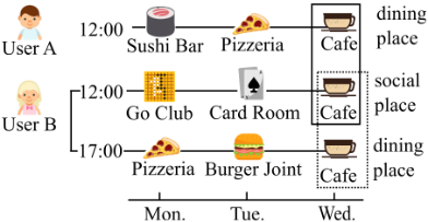
The existing POI recommendation works are mainly based on sequence-based methods, such as [Cheng et al., 2013; Yao et al., 2017; Tang and Wang, 2018], where they regard user's visit history as a sequence. In these methods, they model user and location separately. Therefore, they fail to handle users' personal preference, and fail to capture their dynamic preference. Furthermore, most of these methods regard users' distance/time to location as objective influences, which ignores the personal acceptance to distance/time, and thus limits their recommendation performance.
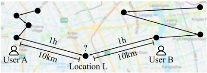
Since Knowledge Graph (KG) can explore heterogeneous graph for multi-relatedness [Wang et al., 2021], some works such as [Wang et al., 2018a; Wang et al., 2019a; Wang et al., 2019b] apply KG in recommendation to learn users' preferences. However, these KG-based methods do not consider temporal information, which makes them can not capture the dynamic changes of users' preferences.
In order to overcome the limitations of the existing sequence-based and KG-based recommendation methods, we introduce Knowledge Graph with temporal information (known as TKG) into POI recommendation, including both user and location with timestamps. In the TKG, we consider users' personal preferences to location and develop attention mechanism to measure each user's acceptance to distance and time. In addition, based on the temporal information in the TKG, we can further learn the dynamic changes of the preferences to enhance the POI recommendation.
Our contributions in this paper are listed as follow:
- We propose a Spatial-Temporal Graph Convolutional Attention Network, a network that learns dynamic relatedness between user/location on a TKG to model users' POI interests. To the best of our knowledge, STGCAN is the first model to explore TKGs to learn users' personal preferences in POI recommendations.
- In STGCAN, we consider users' personal preference for location and construct user/location-receptive-fields respectively on the TKG, to capture the neighbourhoods of user/location for learning representations.
- In STGCAN, we develop an attention mechanism that can measure each user's acceptance to distance and time, such that enhances POI recommendation.
- Experimental results on three real-world datasets show that STGCAN with high personalized characteristics outperforms state-of-the-art baselines, especially in Top1 evaluation.
2 ProblemDescription
Our task is to predict the possible locations for users. Our model's input is user's history visit sequence Y with location GPS information, and TKG G. Our output is a location probability matrix P. Each sequence in the Y contains three attributes (ui, li, ti), which means ui visit li at time ti.
Definition of Temporal Knowledge Graph. The TKG G is represented as quadruple G = {(eu, r, el, t)|eu ∈ Eu, e ∈ R, el ∈ El, t ∈ T}, where eu and el signal the user entity and location entity; relation r represents the strength of the 'Visit' relationship; t is the timestamp when the relatedness happens. G can also be sliced into a set of subgraphs with timestamps, formulated as G = {G1, G2, ..., Gt}.
Definition of Receptive Field. We denote H(D) U/L,U as user/location-receptive-field with D depths; eu′ /l′ as user/location neighbour entity; N u/l as neighbour entity set. The neighbour entity is a relative concept to the target entity.
3 Methodology
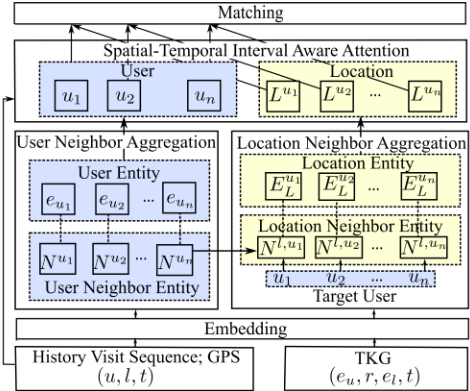
Figure 3 presents the architecture of the proposed STGCAN. STGCAN has four main layers: (1) Embedding Layer (2) User Neighbour Aggregation Layer (3) Location Neighbour Aggregation Layer (4) Spatial-Temporal Interval Aware Attention Layer. The Embedding Layer encodes inputs into latent embeddings. The User/Location Neighbour Aggregation Layers aggregate user/location neighbourhood entities on the TKG. The Spatial-Temporal Interval Aware Attention Layer integrates representations of users/locations with spatial-temporal interval by attention mechanism.
3.1 Embedding Layer
In Embedding Layer, we firstly map the raw timestamps of the history visit sequence Y into 24 × 7 hours (one-hour interval within a week). Then, we encodes the sets of user U, location L, timestamps T into low-dimensional latent embedding metrics: EU ∈ RN×E , EL ∈ RM×E , ET ∈ RK×E , where E is the dimension of the embedding size.
3.2 Neighbour Aggregation Layer
Inspired by the work [Wang et al., 2019a] that combines item neighbourhood for the static representation on KG, we further consider the dynamic representation of both user and location entities on TKG. Specifically, based on the temporal information on the TKG, we aggregate the respective neighbourhood of user and location entities at each timestamp with the constructed user/location-receptive-fields.
User Neighbour Aggregation Layer
User-receptive-field is constructed to aggregate the user neighbour entities on the TKG for user representation.
Firstly, for the quadruple (eu, r, el, t) in G, we define the user neighbour entity eu′ of eu as the entity that shares the same location entity with eu before time t, formed in quadruple (eu′ , r, el, t′ ) (t′ < t). We select the latest K neighbour entities (K can be understood as the neighbour size, which will be evaluated in the experiments) by timestamps, formulated as N u t = {eu′ ,1 t , eu′ ,2 t , ..., eu′ ,K t }. Figure 4 gives an illustrative example of a target user entity with its user neighbour entities on a three-depth user-receptive-field on G.
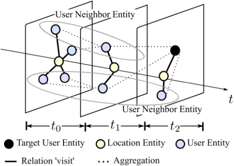
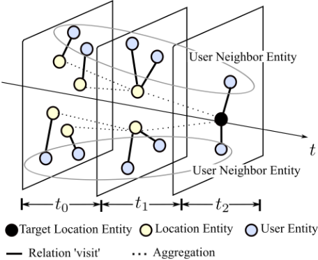
Then, to distinguish the relevance of the K neighbour entities to the target user, the relation r on G is redefined by a spatial-temporal scoring function I, which scores for the relatedness between entities. Function I is further separated into Is and It, which calculate spatial score and temporal score respectively. Here, the spatial score of Is equals to zero because the target user shares the same location with his neighbours. The final spatial-temporal score λu,u′ st outputs as:
where γ is a fine-tuned hyper-parameter. Each user neighbour entity in N u t corresponds to a λu,u′ st score.
Finally, we obtain the K user neighbour entities with dot produce of their softmax-normalized spatial-temporal scores. The target user representation is integrated by the K neighbour entities via a linear transformation, formulated as:
The representation of the target user will thus be updated, and the aggregation process will repeat in every depth of H(D) U :
Location Neighbour Aggregation Layer
Location-receptive-field is constructed to aggregate the neighbour entities on the TKG for location representation. It is worthwhile that, according to users' personal preference for location, the location neighbours will be chosen by user and his neighbours. Specifically, each location has different location neighbours that vary from users.
Figure 5: A target location entity (black) with a three-depth locationreceptive-field on Gt. Firstly, the yellow entities in Gt0 are aggregated to update the yellow entities in Gt1 . Then, those yellow entities in Gt1 are aggregated to update the target black entity in Gt2 . User neighbour entities (purple) help to choose the yellow entities.
Firstly, for the quadruple (eu, r, el, t) in G, we define location neighbour entity el′ of el to user entity eu, as the location entity that be connected with user u's user neighbour entity eu′ before time t, formulated as (eu′ , r, el′ , t′ ) (t′ < t). The connected relation can be understood as 'visit' in semanticity.
Specifically, we concatenate the user neighbour entities N u for each user by sorted timestamps, formulated as N u = concat(N u t |i ∈ T), and then choose the location entity with the latest timestamp ˆ t that is no greater than t as the neighbour location entity, via a lower bound function:
Corresponding to the K user neighbour entities of user u at every specific timestamp, each location will therefore have K location neighbour entities at the same time of user u, formulated as N l,u t = {el′1 ,u t , el′2 ,u t , ..., el′K ,u t }. Figure 5 gives an illustrative example of a location entity with its neighbour entities by a three-depth location-receptive-field of G.
Then, to distinguish the relevance of the K location neighbour entities to the target location, the relation r on G is scored by the similar spatial-temporal scoring function I, in user-receptive-field. Here, we replace the exponent in It with reciprocal operation to enhance the time interval award, and utilize GPS coordinates in Is for calculating haversine distance. The spatial-temporal score for location entity is calcu-
lated as λl,l′u
st = I = Is + It:
Finally, the target location representation is integrated by the representation of itself and its K neighbour entities with similar combination functions in user-receptive-field:
3.3 Spatial-Temporal Interval Aware Attention Layer
After neighbour aggregation, the representations of user and location are then fed into Spatial-Temporal Interval Aware Attention Layer, an attention layer that measures the spatial distance and time interval as the spatial-temporal interval, and assign weights combined relative proportion of both inside the user and between the users to representation.
Firstly, the spatial-temporal interval is calculated by the spatial distance ∆s and time interval ∆t between each sequence with their minimum/maximum values ∆s/tmin/max ∈ RN as the upper/lower bounds: d = dt+ds:
The above trainable parameters vsl, vsu, vtl, vtu ∈ RE , inv s, inv t ∈ RN×E signal the global minimum/maximum spatial/temporal intervals and users' relative spatial/temporal proportion weights. We combine the relative proportion by inner product, for example to spatial interval: vsu · inv s.
Then, we inject the obtained spatial-temporal intervals into the user/location representation by applying self-attention. We incorporate the time embedding into the representation as the attention input, to emphasize the sequential influence. The user/location representations are computed as follow:
where W Q is query matrix, UAtt ∈ RN×M×E , LAtt ∈ RN×L×M×E .
Finally, the visit probability is computed by the cross product of the user and location representation:
3.4 Neural Network Training
The probability distribution of location lj in P can be expressed as p(lj |ui, rm, tk), which indicates the visit probability of user ui to the location lj next to the visit rm at time tk. Algorithm 1 denotes the overall process of network training.
For training, we use cross-entropy as loss function and randomly sample s negative samples at every training step:
Algorithm 1: STGCAN
Input: User history visit sequence Y ; GPS; TKG G
Data: negative sample size s; neighbour entity size
K; receptive field depth H;
Output: Prediction function: P = p(lj|ui, rm, tk) while Network not converge do
Update parameters by gradient descent
| NYC | TKY | Gowalla | |
|---|---|---|---|
| # users | 1,083 | 2,293 | 18,737 |
| # locations | 5,136 | 7,708 | 32,510 |
| # check-ins | 147,938 | 443,477 | 1,496,597 |
Table 1: Details of Datasets
where Θ = {vsu, vsl, vtu, vtl, inv t, inv s,W Q, ...} are learnable parameters and σ is the Sigmoid activity function.
4 Experiments
In this section, we first give a brief introduction to the datasets, the baseline models and the evaluation metrics. We then compare the experimental results of STGCAN with other baselines. Finally, we explore the impacts of different hyperparameter settings to the performance of STGCAN.
4.1 Datasets
We use three public real-world datasets: NYC, TKY and Gowalla, to demonstrate the effectiveness of our model. The three datasets contain user id, location id, timestamp, the latitude and longitude of location. To filter inactive users and locations, in Gowalla dataset, we remove the records of users that have fewer than 20 check-ins and locations that have fewer than 20 visits; in NYC and TKY datasets, we remove the records of users that have fewer than 10 check-ins and locations that have fewer than 10 visits. Table 1 shows the details of the datasets.
The datasets are formed as order sequences by timestamps, where the first [1,m-2) sequences are for training; the (m2)-nd is for validations the (m-1)-st is for test; the [2,m2]-th, (m- 1)-st, m-th sequences are set as the labels of the three parts respectively.
4.2 Baseline Models
We compare our models with the following baselines:
| Model | NYC | TKY | Gowalla | ||||||
|---|---|---|---|---|---|---|---|---|---|
| Recall@1 | Recall@5 | Recall@10 | Recall@1 | Recall@5 | Recall@10 | Recall@1 | Recall@5 | Recall@10 | |
| BPR-MF | 0.074 | 0.148 | 0.224 | 0.079 | 0.179 | 0.260 | 0.046 | 0.128 | 0.155 |
| TransRec | 0.113 | 0.314 | 0.408 | 0.064 | 0.161 | 0.268 | 0.062 | 0.163 | 0.243 |
| Tisasrec | 0.119 | 0.252 | 0.393 | 0.098 | 0.222 | 0.389 | 0.073 | 0.201 | 0.306 |
| Deepmove | 0.134 | 0.300 | 0.374 | 0.124 | 0.288 | 0.341 | 0.098 | 0.200 | 0.275 |
| PRME | 0.157 | 0.385 | 0.476 | 0.117 | 0.318 | 0.416 | 0.089 | 0.209 | 0.267 |
| GeoSAN | 0.167 | 0.401 | 0.544 | 0.125 | 0.316 | 0.371 | 0.106 | 0.277 | 0.364 |
| STAN | 0.181 | 0.412 | 0.593 | 0.133 | 0.326 | 0.397 | 0.109 | 0.302 | 0.400 |
| KGCN | 0.024 | 0.076 | 0.117 | 0.023 | 0.055 | 0.072 | - | - | - |
| CyGNet | 0.207 | 0.413 | 0.586 | 0.109 | 0.294 | 0.406 | 0.112 | 0.311 | 0.385 |
| STGCAN | 0.257 | 0.544 | 0.629 | 0.171 | 0.357 | 0.457 | 0.129 | 0.343 | 0.414 |
| -TKG | 0.171 | 0.471 | 0.587 | 0.129 | 0.328 | 0.428 | 0.096 | 0.268 | 0.349 |
| -ST | 0.209 | 0.513 | 0.619 | 0.161 | 0.384 | 0.449 | 0.107 | 0.228 | 0.314 |
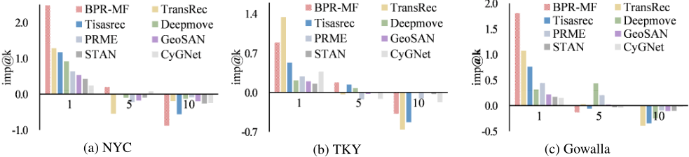
Figure 6: Improvement recall ratios of STGCAN compared with baselines.
- BPR-MF [Rendle et al., 2009]: A Bayesian personalized recommendation model.
- PRME [Feng et al., 2015]: A Markov Chain based personalized recommendation model.
- TransRec [Kang and McAuley, 2018]: A personalized sequential recommendationmodel that considers temporal and spatial contexts in a RNN.
- DeepMove [Zhou and Huang, 2018]: A sequential recommendation model, which captures periodicity in historical sequence and current sequence respectively with attention mechanisms in a RNN.
- KGCN [Wang et al., 2019a]: A KG-based recommendation model, which computes representation with multihop neighbourhoods, but without temporal information.
- TiSASRec [Li et al., 2020]: A sequential recommendation model, which explores explicit time intervals with self-attention, but without spatial information.
- GeoSAN [Lian et al., 2020]: A sequential POI recommendation model, which designs self-attention geography encoder, but lacks personalization.
- STAN [Luo et al., 2021]: A sequential POI recommendation model with bi-attention architectures, but lacks personalization.
- CyGNet [Zhu et al., 2021]: A TKG-based sequential network model with time-aware copy-generation mechanisms, but ignores spatial influence factors.
4.3 EvaluationMetrics and Parameter Settings
To evaluate the performance of our proposed model, we employ Recall@k, a widely used metric. The Recall@k counts the rate of the label in the top {1, 5, 10} probability samples.
To ensure fair comparisons, we initialize the common parameters of baselines with original settings in their papers and fine-tune each model's unique hyperparameters on the experimental datasets. For our model 1 , we set the embedding size to 40, the maximum visit sequence length to 100, the dropout rate of 0.2, and the learning rate of 0.03 in experiments.
4.4 Results
For each model, we perform 10-fold cross-validation, and calculate the average result as the final report. Table 2 shows the performances of all models under Recall@k∈ {1, 5, 10}. Note that, since the Gowalla dataset lacks location category labels, KGCN can not be applied to it, we remove the corresponding result in Table 2. Additionally, to further evaluate the improvement ratios of STGCAN in each k={1, 5, 10} stage, in Figure 6, we compare STGCAN with baselines based on the ratio calculated as follows:
From the results, we can observe that:
1 https://github.com/greenwangzero/STGCAN
| depth | 1 | 2 | 3 |
|---|---|---|---|
| NYC | 0.214 | 0.257 | 0.199 |
| TKY | 0.157 | 0.157 | 0.128 |
| Gowalla | 0.128 | 0.129 | 0.096 |
- In Table 2, the proposed model STGCAN outperforms baselines in all ranges of k in three datasets, which demonstrates the effectiveness of STGCAN for POI recommendation. STGCAN without neighbour aggregation (-TKG) performs low especially in top range of prediction, and STGCAN without spatial-temporal information (-ST) performs low in mostly all ranges of prediction, which shows that the neighbour aggregation and spatial-temporal information in STGCAN have great impacts on the performance.
- In Figure 6, the improvement recall ratio of STGCAN significantly exceed baselines in recall@1 stage, which indicates that STGCAN can learn users' preference well to recommend personalized POIs.
- KGCN and CyGNet are both KG-based models. KGCN performs the worst, and CyGNet performs the best among the baselines. That's because KGCN on KG does not consider the temporal influence, and CyGNet on TKG focuses more on exploring temporal facts. This indicates that, when incorporating KG into a recommendation, temporal influence is a crucial factor.
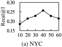
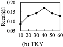
Impact of embedding dimension. In Figure 7, we try the embedding dimension from 10 to 60, and find that STGCAN performes best when it is 40.
Impact of depth of receptive field. In Table 3, we compare different depths of the receptive field in STGCAN. The results show that receptive field can enhance performance, and low depth H = 1 or 2 is enough to achieve good performance, which is also be demonstrated in KGCN [Wang et al., 2019a].
Impact of neighbour entity size. In Table 4, we experiment with the neighbour size of {1, 2, 4, 6} and find that 2 neighbour entities in Gowalla and 4 neighbour entities in NYC and TKY are the best settings. Datasets with more sparse data may be more sensitive to neighbour size because larger neighbour size brings more noise to network.
| neighbour | 1 | 2 | 4 | 6 |
|---|---|---|---|---|
| NYC | 0.145 | 0.228 | 0.257 | 0.199 |
| TKY | 0.114 | 0.157 | 0.171 | 0.129 |
| Gowalla | 0.071 | 0.129 | 0.126 | 0.096 |
5 RelatedWork
5.1 Sequential POI Recommendation
Sequential POI Recommendations model user's history visit as order sequence for POI recommendation. As the existing sequential recommendation methods, Recurrent Neural Networks (RNNs) [Graves, 2008] based methods have been applied with transition matrices [Liu et al., 2016], gates of GRU [Chung et al., 2014; Zhou and Huang, 2018] and LSTM networks [Hochreiter and Schmidhuber, 1997] with variants [Schuster and Paliwal, 1997; Wu et al., 2020]. Although these RNNs-based methods can well preserve dynamic properties of user history, they can not well handle the data sparsity in recommendation, which makes them especially hard to train.
Recently, inspired by attention mechanism in Transformer [Vaswani et al., 2017], attention methods have been applied in sequential recommendation, such as self-attention on users' recent visit sequence [Kang and McAuley, 2018; Wang et al., 2018b], relative time interval [Li et al., 2020], geography encoder [Lian et al., 2020], and bi-layer attention [Luo et al., 2021]. However, these attention-based methods mainly focus on weight-relatedness, but fail to explore graph structure information.
5.2 Knowledge Graph-based Recommendation
To learn graph structure relatedness, some works incorporate Knowledge Graphs into recommendation. [Schlichtkrull et al., 2018] translates recommendation tasks into knowledge base completion tasks; [Wang et al., 2018a; Wang et al., 2019a] use multi-hop neighbourhood structure for representation; [Wang et al., 2019b] employ attention mechanism on entities; [Zhu et al., 2021] focus on time-ware copy factors. However, these methods do not consider the dynamic user preference when exploring KG, and most of them only construct graphs of items.
6 Conclusions
In this paper, we propose a Spatial-Temporal Graph Convolutional Attention Network (STGCAN), which explores spatialtemporal neighbourhood information to model users' POI preferences. In our work, we first construct a TKG with user and location, and then apply user/location-receptive-fields for neighbour aggregation to capture the personalized representation. After that, a Spatial-Temporal Interval Aware Attention Layer is applied to exploit spatial-temporal interval with attention mechanisms. Finally, our experiments on three realworld datasets demonstrate that STGCAN outperforms the state-of-the-art POI recommendation approaches.
Acknowledgements
This work was supported by Shanghai Science and Technology Commission 22YF1401100 and Fundamental Research Funds for the Central Universities 22D111210.
@inproceedings{ijcai2022p490,
  title     = {Modeling Spatio-temporal Neighbourhood for Personalized Point-of-interest Recommendation},
  author    = {Wang, Xiaolin and Sun, Guohao and Fang, Xiu and Yang, Jian and Wang, Shoujin},
  booktitle = {Proceedings of the Thirty-First International Joint Conference on
               Artificial Intelligence, {IJCAI-22}},
  publisher = {International Joint Conferences on Artificial Intelligence Organization},
  editor    = {Luc De Raedt},
  pages     = {3530--3536},
  year      = {2022},
  month     = {7},
  note      = {Main Track},
  doi       = {10.24963/ijcai.2022/490},
  url       = {https://doi.org/10.24963/ijcai.2022/490},
}
TY - CPAPER TI - Modeling Spatio-temporal Neighbourhood for Personalized Point-of-interest Recommendation AU - Wang, Xiaolin AU - Sun, Guohao AU - Fang, Xiu AU - Yang, Jian AU - Wang, Shoujin T2 - Proceedings of the Thirty-First International Joint Conference on Artificial Intelligence, IJCAI-22 PB - International Joint Conferences on Artificial Intelligence Organization PY - 2022 SP - 3530 EP - 3536 DO - 10.24963/ijcai.2022/490 UR - https://doi.org/10.24963/ijcai.2022/490 ER -Copied
Machine-readable versions of this paper, for tools and AI agents:





