
Subsequence-based Graph Routing Network for Capturing Multiple Risk Propagation Processes
Proceedings of the Thirty-First International Joint Conference on Artificial Intelligence. Main Track. Pages 3810-3816.
https://doi.org/10.24963/ijcai.2022/529
Keywords
- Machine Learning: Sequence and Graph Learning
- Multidisciplinary Topics and Applications: Finance
Abstract
In finance, the risk of an entity depends not only on its historical information
but also on the risk propagated by its related peers. Pilot studies rely on Graph Neural Networks (GNNs) to model this risk propagation, where each entity is treated as a node and represented by its time-series information.
However, conventional GNNs are constrained by their unified messaging mechanism with an assumption that the risk of a given entity only propagates to its related peers with the same time lag and has the same effect, which is against the ground truth. In this study, we propose the subsequence-based graph routing network (S-GRN) for capturing the variant risk propagation processes among different time-series represented entities. In S-GRN, the messaging mechanism between each node pair is dynamically and independently selected from multiple messaging mechanisms based on the dependencies of variant subsequence patterns. The S-GRN is extensively evaluated on two synthetic tasks and three real-world datasets and demonstrates state-of-the-art performance.
- [Ali and Hirshleifer, 2020] Usman Ali and David Hirsh- leifer. Shared analyst coverage: Unifying momen- tum spillover effects. Journal of Financial Economics, 136(3):649-675, 2020.
- [Campbell et al., 2010] John Y Campbell, Christopher Polk, and Tuomo Vuolteenaho. Growth or glamour? fundamen- tals and systematic risk in stock returns. The Review of Financial Studies, 23(1):305-344, 2010.
- [Chang et al., 2017] Shiyu Chang, Yang Zhang, Wei Han, Mo Yu, Xiaoxiao Guo, Wei Tan, Xiaodong Cui, Michael J. Witbrock, Mark A. Hasegawa-Johnson, and Thomas S. Huang. Dilated recurrent neural networks. In Advances in Neural Information Processing Systems, pages 77-87, 2017.
- [Cheng and Li, 2021] Rui Cheng and Qing Li. Modeling the momentum spillover effect for stock prediction via attribute-driven graph attention networks. In Proceed- ings of the AAAI Conference on Artificial Intelligence, vol- ume 35, pages 55-62, 2021.
- [Chiu and Nichols, 2016] Jason PC Chiu and Eric Nichols. Named entity recognition with bidirectional lstm-cnns. Transactions of the Association for Computational Lin- guistics, 4:357-370, 2016.
- [Chung et al., 2014] Junyoung Chung, Caglar Gulcehre, KyungHyun Cho, and Yoshua Bengio. Empirical evalua- tion of gated recurrent neural networks on sequence mod- eling. arXiv preprint arXiv:1412.3555, 2014.
- [Chung et al., 2017] Junyoung Chung, Sungjin Ahn, and Yoshua Bengio. Hierarchical multiscale recurrent neural networks. In International Conference on Learning Rep- resentations, 2017.
- [Costello, 2020] Anna M Costello. Credit market disruptions and liquidity spillover effects in the supply chain. Journal of Political Economy, 128(9):3434-3468, 2020.
- [Edwards et al., 2018] Robert D Edwards, John Magee, and WH Charles Bassetti. Technical analysis of stock trends. 2018.
- [Feng et al., 2019] Fuli Feng, Xiangnan He, Xiang Wang, Cheng Luo, Yiqun Liu, and Tat-Seng Chua. Temporal re- lational ranking for stock prediction. ACM Transactions on Information Systems, 37(2):1-30, 2019.
- [Genc ¸ay et al., 2003] Ramazan Genc ¸ay, Faruk Selc ¸uk, and Brandon Whitcher. Systematic risk and timescales. Quan- titative Finance, 3(2):108, 2003.
- [Hochreiter and Schmidhuber, 1997] Sepp Hochreiter and Jürgen Schmidhuber. Long short-term memory. Neural computation, 9(8):1735-1780, 1997.
- [Hou, 2007] Kewei Hou. Industry information diffusion and the lead-lag effect in stock returns. The Review of Finan- cial Studies, 20(4):1113-1138, 2007.
- [Hsu et al., 2021] Yi-Ling Hsu, Yu-Che Tsai, and Cheng-Te Li. Fingat: Financial graph attention networks for recom- mending top-k profitable stocks. IEEE Transactions on Knowledge and Data Engineering, 2021.
- [Jang et al., 2017] Eric Jang, Shixiang Gu, and Ben Poole. Categorical reparameterization with gumbel-softmax. In International Conference on Learning Representations, 2017.
- [Kipf and Welling, 2017] Thomas N. Kipf and Max Welling. Semi-supervised classification with graph convolutional networks. In International Conference on Learning Rep- resentations, 2017.
- [Li et al., 2021] Yongli Li, Chao Liu, Tianchen Wang, and Baiqing Sun. Dynamic patterns of daily lead-lag networks in stock markets. Quantitative Finance, pages 1-14, 2021.
- [Lo et al., 2000] Andrew W Lo, Harry Mamaysky, and Jiang Wang. Foundations of technical analysis: Computational algorithms, statistical inference, and empirical implemen- tation. The Journal of Finance, 55(4):1705-1765, 2000.
- [Menzly and Ozbas, 2010] Lior Menzly and Oguzhan Ozbas. Market segmentation and cross-predictability of returns. The Journal of Finance, 65(4):1555-1580, 2010.
- [Osadchiy et al., 2016] Nikolay Osadchiy, Vishal Gaur, and Sridhar Seshadri. Systematic risk in supply chain net- works. Management Science, 62(6):1755-1777, 2016.
- [Qin et al., 2017] Yao Qin, Dongjin Song, Haifeng Chen, Wei Cheng, Guofei Jiang, and Garrison W. Cottrell. A dual-stage attention-based recurrent neural network for time series prediction. In Carles Sierra, editor, Interna- tional Joint Conference on Artificial Intelligence, pages 2627-2633, 2017. IJCAI
- [Scarselli et al., 2009] Franco Scarselli, Marco Gori, Ah Chung Tsoi, Markus Hagenbuchner, and Gabriele Monfardini. The graph neural network model. IEEE Trans. Neural Networks, 20(1):61-80, 2009.
- [Scholes, 2000] Myron S Scholes. Crisis and risk manage- ment. American Economic Review, 90(2):17-21, 2000.
- [Serrano et al., 2018] Alejandro Serrano, Rogelio Oliva, and Santiago Kraiselburd. Risk propagation through payment distortion in supply chains. Journal of Operations Man- agement, 58:1-14, 2018.
- [Vaswani et al., 2017] Ashish Vaswani, Noam Shazeer, Niki Parmar, Jakob Uszkoreit, Llion Jones, Aidan N Gomez, Łukasz Kaiser, and Illia Polosukhin. Attention is all you need. In Advances in Neural Information Processing Sys- tems, pages 5998-6008, 2017.
- [Xu et al., 2015] Bing Xu, Naiyan Wang, Tianqi Chen, and Mu Li. Empirical evaluation of rectified activations in con- volutional network. CoRR, abs/1505.00853, 2015.
References were extracted automatically from the PDF and may contain errors.
Full text extracted automatically from the PDF; figures, tables and equations may differ. The PDF is the version of record.
1 Introduction
Typically, entities (like stocks) of a financial system (like the stock market) are represented by their time-series information. Since all of the entities are belong to the same ecosystem, the movement of each entity is inevitably affected by peer entities. Such peer influences are called risk propagation in finance [Scholes, 2000; Ali and Hirshleifer, 2020]. Capturing the risk propagation of different time-series is an open problem in many financial applications. The challenge lies in how to define and discover the dependencies of different time-series. To model the risk propagation process, pilot studies apply Graph Neural Networks (GNNs) [Scarselli et al., 2009] by considering the financial system as a graph, where each entity is treated as a node, and edges are defined by certain types of entity relations [Feng et al., 2019]. Specifically, each entity is vectorized by sequentially arranging its information in the past T days. Conventional GNNs (e.g., the GCN [Kipf and Welling, 2017]) use a weight matrix in each layer to discriminate the element importance of a source node vector to generate its message vectors that represent different information (or risk) propagated to others. Given that the risk of a given entity can propagate in variant forms, restricting to a shared weight matrix to express such processes inevitably limits the representation power of conventional GNNs.
∗Corresponding author:liqing@swufe.edu.cn
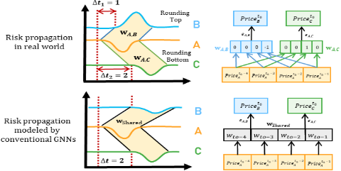
To better understand diverse forms for risk propagation between different time-series, let us take the lead-lag phenomenon of the stock market as an example. The leadlag phenomenon describes that the current price of a given stock is cross-correlated with the "future" prices of its related stocks [Hou, 2007; Menzly and Ozbas, 2010]. Suppose company A is a competitor of B and a sales agent of C. In Figure 1, the declining sale of A leads to a "rounding bottom" trading pattern on its price trend curve. Intuitively, the declining sale of A affects its supplier C, resulting in a falling pattern in the price trend curve of C. However, the downward pressure of A in the stock market may cause an upward price trend of its competitor B. Therefore, the risk of A propagates to B and C, resulting in the appearance of a reverse trading pattern at (i.e., a "rounding top") in the price trend curve of B with a time delay of ∆t1, and a similar trading pattern in C with a time delay of ∆t2 (the lead-lag phenomenon). However, conventional GNNs with shared matrices assume that risks can only propagate with the same time lag and in similar patterns as in Figure 1. This is against the ground truth that various forms of risk propagation exist in time series.
Unfortunately, the forms of risk propagation are implicit and hard to be directly obtained. A promising way is to track risk propagation in terms of the dependencies of subsequence patterns between two time-series. As in the above example, the risk of A to B (or C) can be empirically inferred by analyzing the time dependency of the predefined subsequences (i.e., "rounding top/bottom"). In fact, stock technical analyzers have been explored various subsequences (trading patterns) to capture abnormal stock movements, including "rounds", "triangles", and "wedges" [Lo et al., 2000; Edwards et al., 2018]. However, more trading patterns remain to be explored. A related research area is the study of sequential models that focuses on extracting sequential patterns for downstream tasks. In this study, we argue that the classic sequential models, including the LSTM [Hochreiter and Schmidhuber, 1997] and the GRU [Chung et al., 2014], are inappropriate for the risk propagation task because they value less the dependencies of subsequences. In addition, we provide two well-designed synthetic tasks to support this argument (Section 3.2).
However, the discriminative subsequences that reveal the risk propagation within a given entity pair can be overshadowed by the global risk that makes all entities (timeseries) change similarly. For instance, in the stock market, there are two mainstream driven sources, namely, marketwide and stock-specific information [Genc¸ay et al., 2003; Campbell et al., 2010]. Essentially, stock-specific information (e.g., the declining sale of A) directly affects the target stock (A) and subsequently propagates to its related stocks, resulting in the lead-lag phenomenon, while the market-wide information induces every stock to move simultaneously in the same direction. For example, during the financial crisis in 2008, the market-wide panic dominated the market as investors raced to sell stocks, resulting in a huge drop in all stocks. Recall that the price curve is driven by the joint effect of both market-wide and stock-specific information, the dominance of market-induced movements makes it difficult to detect the trading patterns that reveal the lead-lag phenomenon. Therefore, the removal of the time-series induced by the global risk is vital to capture the dependency of subsequences related to the risk propagation.
In this study, we focus on modeling the risk propagation in the stock market (i.e., the lead-lag phenomenon), since the realistic trading behavior of investors is publicly available and objectively reveals the risk propagation among listed firms. To solve the aforementioned problems, this study proposes the Subsequence-based Graph Routing Network (SGRN) that distinguishes itself with three main modules:
- To model the variant forms of risk propagation, we propose the Graph Routing Network (GRN) which extends conventional graph neural networks with multiple messaging parameter sets, and the Messaging Mechanism Router (MMR) that selects the optimal one for each stock pair dynamically and independently.
- To felicitate the selection process of GRN, we mingled it with the Subsequence Detector (SD), which learns to generate latent boundaries for discriminative subsequences and encodes the dependencies of their combinations and time lags into sequential embeddings.
- To eliminate the impact of global risk on individual stock movements, the Market-wide Risk Separator (MRS) is proposed to split the original stock movement into the market-induced and the stock-specific movement by measuring its temporal similarity with the market trend.
Experiments conducted on S&P500 stocks in three different periods (i.e., bullish, bearish, and sideways) show the superiority of the S-GRN over the state-of-the-art algorithms. In addition, two synthetic tasks are designed to demonstrate the reason that the proposed sequential module is better than the classic sequential models including LSTM and GRU lies in its capability of detecting dependencies of subsequences related to risk propagation.
2 Model Architecture
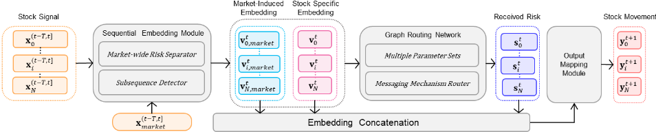
Figure 2 is an overview of the S-GRN. First, the MRS divides the original stock movement into the market-induced and the stock-specific movement, and the SD separately generates their sequential embeddings that encode the combinations and time lags of subsequences related to downstream tasks. The stock-specific sequential embeddings are then utilized by the Graph Routing Network (GRN) to generate the relational embeddings that represent risks received by stocks. The MMR of the GRN selects the optimal parameter set for propagating risk between each stock-pair independently and dynamically based on the dependencies of trading patterns detected in their recent price curves. Lastly, for a given stock, its market-induced, stock-specific, and relational embeddings are combined to predict its future movement via the Output Mapping module. In the following, we use x (lower-case letter) to denote a scalar, x (bold lower-case letter) to denote a vector, X (upper-case letter) to denote a matrix.
2.1 Sequential EmbeddingModule
Subsequence Detector (SD)
Many researches have adopted variant RNNs (i.e., the LSTM and the GRU) to capture the temporal dependencies of technical indicators for stock prediction [Feng et al., 2019; Cheng and Li, 2021; Hsu et al., 2021]. For a given stock i in day t, the RNNs are expected to generate its F-dimensional sequential embedding, vt i ∈ RF , that benefits downstream tasks using its L-dimensional time series features, xti ∈ RL, in the past T days, x(t-T,t] i = [xt-T+1 i , . . . , xti ].
As illustrates in previous examples, multiple sub-trading patterns (subsequences) exist in a given look-back window of size T, and their combinations and time lags are critical for downstream tasks. However, as proved in our synthetic tasks (refer to Section 3.2), the ability to detect such information is insufficient in the LSTM and the GRU. Although the LSTM and the GRU have achieved great success in sequence segmentation tasks, such as named-entity recognition [Chiu and Nichols, 2016], where the subsequence boundary is explicitly given, it is impractical for human beings to formally define and manually label the boundary between different implicit trading patterns associated with downstream tasks. Inspired by [Chung et al., 2017], the SD learns to detect the latent subsequence boundary based on supervising signals in downstream tasks via the Subsequence-aware LSTM.
In conventional LSTMs, for a given cell in layer l at time t, the inputs from its lower layer, htl-1 , and the hidden state of its last time step, ht-1 l , are used to calculate its forget gate (f t l ), input gate (itl ), output gate (otl ), and candidate gate ˜ctl , which are then used to update its cell state (ctl ) and hidden state (htl ). In addition to these gates, the subsequence-aware LSTM additionally generates a binary value, zt l , to represent the end of a detected subsequence (or the boundary between subsequences).
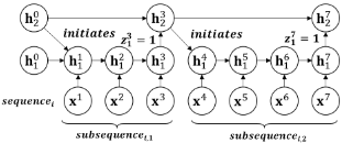
Figure 3 shows an example of applying a two-layer Subsequence-aware LSTM to a sequence consisting of two subsequences. When the subsequence1 is detected in layer 1 at time 3 (z3 1 = 1), its summary representation (h31 ) is propagated to the upper layer before being erased. The next hidden state of the current layer, h41 , instead of being updated by h31 as in the conventional LSTM, is reinitialized for subsequence2 using h32 that contains long-term information. For cells in layer 2, their hidden states are updated only when the summary representations of subsequences (i.e., h31 and h71 ) are propagated from layer one, otherwise they will remain unchanged.
As introduced in the previous example, the cell in layer l at time t of Subsequence-aware LSTM will erase previous hidden state, ht-1 l , and be reinitialized with the input from the upper layer, ht-1 l+1 , if the end of a subsequence is detected in previous cell (zt-1 l = 1). The cell will consider the input from lower layer, htl-1 , only if it is the summary representation of a subsequence (ztl-1 = 1). Therefore, in Subsequence-aware LSTM, the cell first obtains its values of the gates (itl , f t l , otl , and ˜ctl ), and the activation value of the newly introduced boundary detector, ˜ zt l , based on two boundary states, i.e., zt-1 l and zt l-1 :
where htl ∈ RF , W i j ∈ R(4F+1)×F is the weight matrix from layer i to layer j, and fslice(·) simply slices the input vector into five parts with dimension sizes [F, F, F, F, 1] and assigns them to itl , ftl , otl , ˜ctl ∈ RF , and ˜ zt l ∈ R, respectively. Then, the cell updates its cell state by:
and last obtains its hidden state by:
where ctl ∈ RF , and ⊗ represents the element-wise multiplication. The binary state zt l that indicates the end of a subsequence is obtained by applying a step function to ˜ zt l :
Due to the non-differentiability of the step function, the hard sigmoid function, h sigm(x) = max(0,min(1, αx+1 2 )), is used in practice, because it can approximate the step function when the slope α is large.
The last layer L of the Subsequence-aware LSTM contains the boundaries of highest-level subsequences, ztL, and their summary representations {htL|ztL = 1}. The combinations and time lags of these detected subsequences could facilitate downstream tasks, which is captured by applying a Transformer with the positional encoding [Vaswani et al., 2017]:
whose last element, vt i ∈ RF , is considered as the sequential embedding of stock i.
Market-wide Risk Separator (MRS)
The market-induced and stock-specific movement alternately dominates the market, and conventional RNNs are unable to capture robust patterns associated with downstream tasks without considering them separately. To distinguish the stock-specific movement from the market-induced movement and learn their trading patterns separately, the MRS first applies a bidirectional LSTM (BiLSTM(·)) to the original time series features of stock i, x(t-T,t] i , to capture its Ldimensional trading context in each time t:
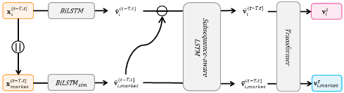
Meanwhile, the MRS also generates another L-dimensional vector that measures the trading context similarity between the original time series features of stock i, x(t-T,t] i , and that of the entire market, x(t-T,t] market , in each time t, by concatenating them into a compound vector and feeding into another BiLSTM (BiLSTMsim(·)):
Then, ˜v(t-T:t] i,market and ˜v(t-T:t] i - ˜v(t-T:t] i,market are considered as the market-induced movement and stock-specific movement of stock i, respectively. They are further fed into the SD to generate market-induced and stock-specific sequential embeddings, vt i,market and vt i , respectively.
Figure 4 shows the whole process of the proposed sequential embedding module. In practice, the market-wide information is obtained by averaging time-series features of all stocks in the market, xtmarket = 1N ∑Ni=1 (xti ). Therefore, the S-GRN doesn't require to use market indexes as input.
2.2 Graph Routing Network
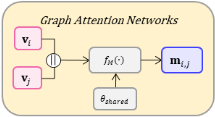
To model the risk propagations, the stock market can be treated as a graph G = (V,E), where V = [v1, . . . , vN] ∈ RN×F is the representation of N stocks, and E ∈ RN×N is the predefined relation of stocks, whose indexes are stocks and elements are their connection strengths. For a target node i and a source node j, the messaging mechanism (fM(·)) in the GAT is adopted by pilot studies to calculate the Fdimensional messages from j to i:
where θ is the learned parameters in fM(·). In a specific layer l ∈ L of GAT, it usually takes the form of:
where θl = (W l s ∈ RF×F ,wle ∈ R(2F+1)×1 ) is the messaging parameter shared by all node pairs in layer l and θ = [θ1 , . . . , θL] is the messaging parameter set in the GAT.
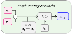
However, as the example illustrated in Figure 1, A's risk propagates to others with different forms, suggesting the existence of variant messaging processes that are mutually exclusive and impossible to be modeled by the shared Ws or θ. To solve this problem, we propose the GRN which contains K different messaging parameter sets, Θ = [θ1, . . . , θK], and the Messaging Mechanism Router (MMR) to select the messaging parameter set, θi,j ∈ Θ, that best describes the specific risk propagation form between j and i. Figure 5 shows its difference with conventional GATs.
Figure 5: Comparing the S-GRN with conventional GATs
Given two stocks, the dependencies of trading patterns imply their risk propagation mechanism [Li et al., 2021]. Therefore, their sequential embeddings generated by the newly proposed sequential module, vt i and vtj , which encode the combination and time lag of discriminative trading patterns, are fed into the MMR to generate the matching scores for the K different messaging parameter sets, ˜ati,j ∈ RK , via a nonlinear function π(·):
which, for simplicity, takes the form of a single-layer MLP activated by the LeakyReLU [Xu et al., 2015]:
To give discrete selection of θ that really distinguishes different lead-lag effects, the straightforward approach is using argmaxj (˜ati,j ) that is not differentiable. To achieve differentiable but discrete selection, we utilize the Gumbel-Softmax trick [Jang et al., 2017] to enable the differentiability of the MMR. Essentially, it adds the Gumbel noises to the matching scores and uses the re-parametrization trick to make the computation fully differentiable:
where ϵ = [ϵ1, ϵ2, . . . , ϵK] are i.i.d. sampled drawn from Gumbel(0, 1)7 distribution and τ is the temperature that controls the sharpness of the output distribution. The θi,j used to obtain the message from j to i is selected by:
and the F dimensional relational embedding of stock i is represented by summing over all its received risks:
2.3 Output MappingModule
Finally, a single-layer feed-forward neural network is applied to generate the prediction of future stock prices ˆ yt+1 i :
where wi ∈ R3F , and bi ∈ R. The Mean Squared Error (MSE) loss between ˆ yt and yt is back-propagated to learn the parameters of the proposed framework.
3 Experimental Evaluation
In this section, we first conduct experiments with real stock market data and compare the S-GRN with state-of-the-art stock prediction frameworks. In addition, through the ablation study, we verify the effectiveness of the three main modules of the S-GRN. Lastly, two synthetic tasks are designed to evaluate the capability of the proposed sequential embedding module in detecting the lead-lag phenomenon.
3.1 Stock Prediction
Dataset
The experiment is conducted on the daily stock transaction data of S&P 500 companies at three testing periods, i.e., when the market is bullish (01/08/2019-01/02/2020), bearish (01/12/2008-1/6/2009), and sideways (01/12/201501/6/2016). For each testing period, the transaction data in the past 5 years is used for training and validation. The transaction data is obtained from the Center for Research in Security Prices. Sixteen technical indicators (features) are derived from the transaction data. We used the supply chain relationship collected from S&P Capital IQ to form the graph edge, since it has proven to be one of the most effective relations for tracking the spread of risk [Osadchiy et al., 2016; Serrano et al., 2018; Costello, 2020].
Evaluation Metrics
The prediction of stock return is studied as a regression task. Therefore, the Mean Square Error (MSE) of the predictions of all stocks and all trading days during the testing period is adopted to evaluate model performance. Expecting that stocks with higher predicted prices should have a higher probability to perform better in the future, we also use the Mean Reciprocal Rank (MRR). It is calculated by first finding the rank of the actual most profitable stock in the prediction on each trading day, and then calculating the average of its reciprocal over the test period. Meanwhile, we also build an equally-weighted portfolio by longing stocks with top 50 predicted returns in each day and report its annualized returns in excess of the S&P 500 index (AER).
Comparisons
We compare the S-GRN with four widely-applied sequential models, i.e., the LSTM, BiLSTM, and DA-RNN [Qin et al., 2017]. In addition, we also compare S-GRN with two stateof-the-art frameworks for the stock prediction task that use the GCN/GAT to model the inter-firm interactions:
- TGC: it combines the LSTM with the GCN for stock prediction. The strength of predefined stock relation in the GCN is adjusted based on the similarity of timeseries features [Feng et al., 2019].
- FinGAT: it combines the LSTM with a variant of GAT with a two-stage attention mechanism [Hsu et al., 2021].
Table 1 shows the average stock prediction performance of all models in 10 different initializations. The graph-based baseline models that consider the risk propagation in the stock market, i.e., TGC and FinGAT, perform better than the sequential models. The S-GRN further improves their performance with the three proposed modules under different testing periods. Here, lower MSE indicates that the model predicts future stock returns with greater confidence. On average over the three periods, it reduces MSE by at least 12.9% and improves MRR by at least 35% compared to the baseline models. Meanwhile, over 3 different periods, it brings an extra 1.3% AER. The result suggests that the core mechanism of S-GRN, i.e., the dynamical and independent selection of the risk propagation process between different stock pairs based on their fine-grained trading pattern detection, is critical in modeling the lead-lag phenomenon for stock prediction.
| Model | Bullish | Bearish | Sideways | ||||||
|---|---|---|---|---|---|---|---|---|---|
| MSE | MRR | AER | MSE | MRR | AER | MSE | MRR | AER | |
| LSTM | 5.13e-4 | 1.1e-2 | -4.3% | 2.51e-3 | 1.1e-2 | 4.8% | 4.81e-4 | 2.0e-2 | 1.4% |
| BiLSTM | 5.03e-4 | 1.1e-2 | -2.6% | 2.73e-3 | 1.1e-2 | 3.9% | 4.92e-4 | 2.1e-2 | -0.8% |
| DA-RNN | 4.57e-4 | 1.3e-2 | -1.4% | 2.30e-3 | 1.2e-2 | 6.3% | 4.63e-4 | 2.3e-2 | 0.7% |
| TGC | 3.73e-4 | 2.2e-2 | 1.3% | 2.52e-3 | 1.5e-2 | 5.0 % | 4.12e-4 | 2.7e-2 | 2.2% |
| FinGAT | 3.62e-4 | 2.1e-2 | 1.7% | 2.40e-3 | 1.4e-2 | 7.3 % | 4.17e-4 | 2.5e-2 | 1.7% |
| Our Method | 2.90e-4 | 2.7e-2 | 1.8% | 2.16e-3 | 2.4e-2 | 10.7% | 3.59e-4 | 3.0e-2 | 3.4% |
Ablation Study
We further determine the effectiveness of the different modules of the S-GRN by conducting an ablation study. The stock trading data in the bearish period is selected, as all stocks are highly exposed to the market-wide risk during this period. The effectiveness of the sequential module of the S-GRN is judged using three of its variants:
- BiLSTM: the vanilla BiLSTM (with 6 layers) that is used in pilot works.
- MRS + BiLSTM: the SD is replaced by a 4-layer BiLSTM, which means the combination and time lag of subsequences is not explicitly modeled.
- BiLSTM + SD: the MRS is replaced by a 2-layer BiLSTM, which means the influence of global risk on individual stocks is not filtered out.
The GRN is judged under two different settings, i.e., K = 1 and K = 5. Note that when K = 1, the MMR of the GRN is removed, and the GRN is downgrade to the GAT.
We have two main observations from Table 2. Firstly, extending conventional GNNs with multiple messaging parameter sets (K) improves the stock prediction performance of S-GRN, which corroborates the claim in recent finance studies that variant forms of risk propagation exist in the stock market, and it is impossible to represent them by one shared messaging parameter set. Secondly, when the ability of the sequential module is limited (e.g., only use the BiLSTM), the GRN (K = 5) can only bring relatively small enhancement in terms of MSE. The result suggests that to select the optimal parameter set for risk propagation, the selection of GRN requires a powerful sequential module that is capable to encode the dependency of subsequences.
3.2 Synthetic Tasks
We create two dummy datasets to further explore the reasons that the proposed sequential module outperforms conventional models in stock prediction 1 . Each sample in the dataset consists of two sequences that represent the marketinduced and stock-specific movement, respectively. The market-induced sequence is generated by drawing 100 numbers independently from the uniform distribution, U(-1, 1). The stock-specific sequence is generated in the same way with an extra operation that a number of predefined subsequences (each consists of 10-15 random numbers) are randomly selected to replace some parts of the sequence.
| Model | K = 1 | K = 5 | ||||
|---|---|---|---|---|---|---|
| MSE | MRR | AER | MSE | MRR | AER | |
| BiLSTM | 2.25e-3 | 1.5e-2 | 4.4% | 2.22e-3 | 1.7e-2 | 5.7% |
| MRS + BiLSTM | 2.24e-3 | 1.6e-2 | 6.5% | 2.17e-3 | 2.2e-2 | 7.5% |
| BiLSTM+ SD | 2.18e-3 | 1.7e-2 | 5.3% | 2.23e-3 | 2.3e-2 | 5.1% |
| MRS + SD | 2.17e-3 | 2.0e-2 | 7.9% | 2.16e-3 | 2.4e-2 | 10.9% |
With 6 manually predefined subsequences, we propose two multi-classification tasks:
1) Given that the risk can propagate in similar or different forms, the 6 predefined subsequences are evenly divided into 3 pattern groups, and samples with the same combination of groups, although the actual subsequences can be different, belong to the same class. In task 1 (T1), models are required to recognize the combination of pattern groups in each stock-specific sequence. 3 predefined patterns are randomly selected to replace different parts of the stock-specific sequence (27 classes).
2) The risk can also propagate in different time lags. In task 2 (T2), models are required to identify the time lags between predefined subsequences appeared in the stock-specific sequence. 2 predefined patterns are randomly selected and their time lag is selected from {5, 10, 15, 20, 25, 30}. Samples with the same time lag between predefined subsequences belong to the same class (6 classes). Each class in the corresponding dataset consists of 300 samples and models are evaluated under 2 input settings:
- Firm Only: the stock-specific sequence of each sample is directly fed into models.
- Firm and Market: the stock-specific sequence is added by the market-induced sequence with a probability of 50% before being fed into models.
Note that, the MRS in the proposed sequential module is equivalent to a 2-layer BiLSTM in processing the input.
We adopt LSTM and BiLSTM as our baseline since both of them are widely used as the sequential module in previous graph-based stock prediction frameworks [Feng et al., 2019; Hsu et al., 2021]. In addition, we also compared with HMLSTM [Chung et al., 2017] and D-LSTM [Chang et al., 2017]. Each model is connected to a single-layer MLP with the softmax activation function that maps its output to the prediction of different classes. The cross-entropy loss between the predictions and true labels is back-propagated to learn the parameters in each model. For each model, we search its optimal number of layer ∈ (1, 6), hidden size ∈ {10, 20, 30}, and learning rate ∈ {1e - 3, 5e - 4, 1e - 4, 5e - 5, 1e - 5}, and trained it with a maximum epoch of 200.
1 https://github.com/RuichengFIC/SGRN
| Model | Firm Only | Firm + Market | with MRS | |||
|---|---|---|---|---|---|---|
| T1 | T2 | T1 | T2 | T1 | T2 | |
| LSTM | 0.55(0.24) | 0.62(0.18) | 0.57(0.17) | 0.55(0.28) | 0.73(0.07) | 0.79(0.12) |
| BiLSTM | 0.79(0.04) | 0.90(0.08) | 0.77(0.08) | 0.74(0.18) | 0.79(0.10) | 0.84(0.15) |
| HM-LSTM | 0.60(0.14) | 0.68(0.10) | 0.55(0.17) | 0.57(0.13) | 0.74(0.08) | 0.80(0.11) |
| D-LSTM | 0.70(0.13) | 0.66(0.15) | 0.64(0.17) | 0.60(0.20) | 0.79(0.07) | 0.78(0.12) |
| Our Method | 0.84(0.04) | 0.98(0.01) | 0.73(0.08) | 0.98(0.01) | 0.92(0.03) | 0.99(0.01) |
Table 3 shows the average and standard deviation of the accuracy of all models in 10-fold cross-validation. The proposed sequential module achieves the best performance in terms of accuracy in all tasks, improving the accuracy by at least 5.0% and 8.0% in T1 and T2, respectively. The result suggests that the insufficient ability of conventional RNNs to capture the combinations and time lags of subsequences could be one of the reasons for their ineffectiveness in predicting the real stock market.
In addition, the performance of all the models suffers a huge decline when the stock-specific sequence is potentially disturbed by the market-induced sequence. This implies that it is difficult to detect discriminative sequential patterns associated with downstream tasks without eliminating sequential patterns caused by the global risk.
Therefore, we further incorporate all models with the MRS that is able to detect and separate the interference caused by adding the market-wide sequence randomly (With MRS). The MRS additionally takes the market-induced sequence as input, since the average of time-series of all listed firm is easy to obtain in practice. Models take the stock-specific embedding generated by MRS as input and are jointly trained with the MRS.
The result shows that, when combined with the MRS, models achieve better performance on different tasks. This suggests that the MRS is able to separate the market-induced movement, and this ability benefits the identification of noise that inherently exists in the stock-specific movement.
4 Conclusion
In this study, we propose the subsequence-based graph routing network (S-GRN) for capturing the variant risk propagation processes among different time-series represented entities. Extensive experiments have demonstrated the superiority of three key mechanisms in S-GRN: 1) determine the risk propagation process for each node pair independently, 2) identify discriminative subsequences and encode their combinations and time lags for downstream tasks, and 3) remove the impact of global risks to better detect sequential patterns that reflect the interconnections between specific entity pairs. These mechanisms can be combined with conventional GNNs applied to recommender systems, fraud detection, etc. However, their effectiveness is yet to be explored.
Acknowledgements
This work was supported by the National Natural Science Foundation of China (NSFC) (71671141, 71873108, and 62072379), the Department of Science and Technology of Sichuan Province (2019YJ0250 and 2020ZYD018), and the Key Laboratory of Financial Intelligence and Financial Engineering of Sichuan Province.
@inproceedings{ijcai2022p529,
  title     = {Subsequence-based Graph Routing Network for Capturing Multiple Risk Propagation Processes},
  author    = {Cheng, Rui and Li, Qing},
  booktitle = {Proceedings of the Thirty-First International Joint Conference on
               Artificial Intelligence, {IJCAI-22}},
  publisher = {International Joint Conferences on Artificial Intelligence Organization},
  editor    = {Luc De Raedt},
  pages     = {3810--3816},
  year      = {2022},
  month     = {7},
  note      = {Main Track},
  doi       = {10.24963/ijcai.2022/529},
  url       = {https://doi.org/10.24963/ijcai.2022/529},
}
TY - CPAPER TI - Subsequence-based Graph Routing Network for Capturing Multiple Risk Propagation Processes AU - Cheng, Rui AU - Li, Qing T2 - Proceedings of the Thirty-First International Joint Conference on Artificial Intelligence, IJCAI-22 PB - International Joint Conferences on Artificial Intelligence Organization PY - 2022 SP - 3810 EP - 3816 DO - 10.24963/ijcai.2022/529 UR - https://doi.org/10.24963/ijcai.2022/529 ER -Copied
Machine-readable versions of this paper, for tools and AI agents:





