
FOGS: First-Order Gradient Supervision with Learning-based Graph for Traffic Flow Forecasting
Proceedings of the Thirty-First International Joint Conference on Artificial Intelligence. Main Track. Pages 3926-3932.
https://doi.org/10.24963/ijcai.2022/545
Keywords
- Data Mining: Mining Spatial and/or Temporal Data
- Multidisciplinary Topics and Applications: Transportation
Abstract
Traffic flow forecasting plays a vital role in the transportation domain.
Existing studies usually manually construct correlation graphs and design sophisticated models for learning spatial and temporal features to predict future traffic states.
However, manually constructed correlation graphs cannot accurately extract the complex patterns hidden in the traffic data.
In addition, it is challenging for the prediction model to fit traffic data due to its irregularly-shaped distribution.
To solve the above-mentioned problems, in this paper, we propose a novel learning-based method to learn a spatial-temporal correlation graph, which could make good use of the traffic flow data.
Moreover, we propose First-Order Gradient Supervision (FOGS), a novel method for traffic flow forecasting.
FOGS utilizes first-order gradients, rather than specific flows, to train prediction model, which effectively avoids the problem of fitting irregularly-shaped distributions. Comprehensive numerical evaluations on four real-world datasets reveal that the proposed methods achieve state-of-the-art performance and significantly outperform the benchmarks.
- [Bai et al., 2019] Lei Bai, Lina Yao, Salil S. Kanhere, Xi- anzhi Wang, and Quan Z. Sheng. Stg2seq: Spatial- temporal graph to sequence model for multi-step passen- ger demand forecasting. In IJCAI, 2019.
- [Chen et al., 2001] Chao Chen, Karl Petty, Alexander Sk- abardonis, Pravin Varaiya, and Zhanfeng Jia. Freeway performance measurement system: Mining loop detector data. TRR, 2001.
- [Fang et al., 2019] Shen Fang, Qi Zhang, Gaofeng Meng, Shiming Xiang, and Chunhong Pan. Gstnet: Global spatial-temporal network for traffic flow prediction. In IJ- CAI, 2019. IJCAI
- [Fang et al., 2021] Zheng Fang, Qingqing Long, Guojie Song, and Kunqing Xie. Spatial-temporal graph ODE net- works for traffic flow forecasting. In KDD, 2021.
- [Gong et al., 2020] Yongshun Gong, Zhibin Li, Jian Zhang, Wei Liu, and Jinfeng Yi. Potential passenger flow predic- tion: A novel study for urban transportation development. In AAAI, 2020.
- [Grover and Leskovec, 2016] Aditya Grover and Jure Leskovec. node2vec: Scalable feature learning for networks. In ACM SIGKDD, 2016.
- [Guo et al., 2019] Shengnan Guo, Youfang Lin, Ning Feng, Chao Song, and Huaiyu Wan. Attention based spatial- temporal graph convolutional networks for traffic flow forecasting. In AAAI, 2019.
- [Han et al., 2021] Peng Han, Jin Wang, Di Yao, Shuo Shang, and Xiangliang Zhang. A graph-based approach for trajec- tory similarity computation in spatial networks. In ACM SIGKDD, 2021.
- [He and Shin, 2020] Suining He and Kang G. Shin. Towards fine-grained flow forecasting: A graph attention approach for bike sharing systems. In WWW, 2020.
- [Li and Zhu, 2021] Mengzhang Li and Zhanxing Zhu. Spatial-temporal fusion graph neural networks for traffic flow forecasting. In AAAI, 2021.
- [Li et al., 2018] Yaguang Li, Rose Yu, Cyrus Shahabi, and Yan Liu. Diffusion convolutional recurrent neural net- work: Data-driven traffic forecasting. In ICLR, 2018.
- [Li et al., 2021] Mingqian Li, Panrong Tong, Mo Li, Zhong- ming Jin, Jianqiang Huang, and Xian-Sheng Hua. Traffic flow prediction with vehicle trajectories. In AAAI, 2021.
- [Liu et al., 2021] Hao Liu, Qiyu Wu, Fuzhen Zhuang, Xin- jiang Lu, Dejing Dou, and Hui Xiong. Community-aware multi-task transportation demand prediction. In AAAI, 2021.
- [Lv et al., 2015] Yisheng Lv, Yanjie Duan, Wenwen Kang, Zhengxi Li, and Fei-Yue Wang. Traffic flow prediction with big data: A deep learning approach. TITS, 2015.
- [Mikolov et al., 2013] Tomás Mikolov, Ilya Sutskever, Kai Chen, Gregory S. Corrado, and Jeffrey Dean. Distributed representations of words and phrases and their composi- tionality. In NIPS, 2013.
- [Song et al., 2020] Chao Song, Youfang Lin, Shengnan Guo, and Huaiyu Wan. Spatial-temporal synchronous graph convolutional networks: A new framework for spatial- temporal network data forecasting. In AAAI, 2020.
- [Wu and Tan, 2016] Yuankai Wu and Huachun Tan. Short- term traffic flow forecasting with spatial-temporal correla- tion in a hybrid deep learning framework. CoRR, 2016.
- [Wu et al., 2019] Zonghan Wu, Shirui Pan, Guodong Long, Jing Jiang, and Chengqi Zhang. Graph wavenet for deep spatial-temporal graph modeling. In IJCAI, 2019. IJCAI
- [Yao et al., 2018a] Huaxiu Yao, Xianfeng Tang, Hua Wei, Guanjie Zheng, Yanwei Yu, and Zhenhui Li. Modeling spatial-temporal dynamics for traffic prediction. CoRR, 2018.
- [Yao et al., 2018b] Huaxiu Yao, Fei Wu, Jintao Ke, Xianfeng Tang, Yitian Jia, Siyu Lu, Pinghua Gong, Jieping Ye, and Zhenhui Li. Deep multi-view spatial-temporal network for taxi demand prediction. In AAAI, 2018.
- [Ye et al., 2021] Junchen Ye, Leilei Sun, Bowen Du, Yanjie Fu, and Hui Xiong. Coupled layer-wise graph convolution for transportation demand prediction. In AAAI, 2021.
- [Yu et al., 2017] Rose Yu, Yaguang Li, Cyrus Shahabi, Ugur Demiryurek, and Yan Liu. Deep learning: A generic ap- proach for extreme condition traffic forecasting. In ICDM, 2017.
- [Yu et al., 2018] Bing Yu, Haoteng Yin, and Zhanxing Zhu. Spatio-temporal graph convolutional networks: A deep learning framework for traffic forecasting. In IJCAI, 2018. IJCAI
- [Zhang et al., 2017] Junbo Zhang, Yu Zheng, and Dekang Qi. Deep spatio-temporal residual networks for citywide crowd flows prediction. In AAAI, 2017.
- [Zhang et al., 2020] Junbo Zhang, Yu Zheng, Junkai Sun, and Dekang Qi. Flow prediction in spatio-temporal net- works based on multitask deep learning. TKDE, 2020.
- [Zhou et al., 2018] Xian Zhou, Yanyan Shen, Yanmin Zhu, and Linpeng Huang. Predicting multi-step citywide pas- senger demands using attention-based neural networks. In WSDM, 2018.
- [Zhou et al., 2021] Qiang Zhou, Jingjing Gu, Xinjiang Lu, Fuzhen Zhuang, Yanchao Zhao, Qiuhong Wang, and Xiao Zhang. Modeling heterogeneous relations across multiple modes for potential crowd flow prediction. In AAAI, 2021.
References were extracted automatically from the PDF and may contain errors.
Full text extracted automatically from the PDF; figures, tables and equations may differ. The PDF is the version of record.
1 Introduction
Traffic flow prediction is one of the most fundamental techniques for intelligent transportation management and services (e.g., route planning, intelligent traffic light control, etc.) [Wu and Tan, 2016; Zhang et al., 2020; He and Shin, 2020]. Accurate prediction of future traffic conditions may help people make travel arrangements, avoid potential congestion in the streets, and wisely allocate transportation resources [Zhang et al., 2017; Zhou et al., 2021; Zhou et al., 2018; Gong et al., 2020; Liu et al., 2021]. Typically, traffic flow prediction relies on traffic flow sensors, which are devices distributed in the road network monitoring the presence or passage of vehicles. A sensor records traffic flows at a fixed frequency (e.g., every 5 minutes), thus generating a sequence of traffic flows over time. Essentially, the data adopted for prediction is a sequence of traffic flow signals, where each signal contains the traffic flows recorded by all the sensors in the road network during some time intervals. The task of traffic flow prediction is naturally spatiotemporal: to predict the future flows of some sensors [Lv et al., 2015; Yu et al., 2017; Bai et al., 2019; Yao et al., 2018a; Yao et al., 2018b] , one may need to consider the flows in the past as well as spatial correlations such as geographical distances to nearby sensors, and structure of the road network.
∗ Indicates equal contribution
†Corresponding Author
Many approaches [Fang et al., 2019; Li et al., 2021; Ye et al., 2021; Wu et al., 2019; Fang et al., 2021] have been proposed for traffic flow prediction. In a nutshell, these methods first build a correlation graph between sensors and then make traffic flow predictions based on the correlation graph. STGCN [Yu et al., 2018] directly uses the road network to describe the spatial correlations between sensors and uses a graph convolution method to extract spatiotemporal features. STSGCN [Song et al., 2020] explicitly establishes temporal correlations between sensors in consecutive traffic flow signals and then uses graph embedding techniques for flow prediction. Recently, [Li and Zhu, 2021] models correlations between sensors via similarities between their flow time series. They construct a fusion graph to reflect both temporal and spatial correlations and propose a gated dilated CNN module for flow prediction.
Although existing methods have made achievements in their own lines of research, we observe the following issues:
- Graph building. Most existing methods fail to make full use of the temporal information in the traffic data. They either completely ignore the historical flows or merely use some overall temporal similarity between them. There lacks consideration on temporal similarity of historical flows at finer granularities. Moreover, most existing correlation graphs are manually built, thus human experience may largely bias the prediction.
- Prediction making. Most existing methods aim to predict the exact traffic flows. The task is challenging as the distribution of traffic flows is irregularly shaped. Us-
ing a limited amount of training data usually causes the problem of under-fitting, which may degrade the accuracy of flow prediction.
In this paper, we aim to tackle the above issues. To make better use of the temporal information, we observe that the traffic flow usually follows a regular weekly pattern, reflecting human activities in weekdays and weekends, rush hours and regular hours, etc. Based on this observation, we decompose a week into a sequence of consecutive time slots, each corresponding to a specific time interval (e.g., 0:00 to 0:05 A.M. on Wednesday) in a week. For each sensor, we construct a temporal feature vector, where each element is the average of the historical flows within the corresponding time slot. The distance between two temporal feature vectors is thereby a similarity measure between the corresponding sensors. With such a similarity measure, we build a temporal correlation graph by linking each sensor with its k most similar sensors. Then, we propose a novel learning-based approach to learn an embedding of each sensor, considering both the temporal correlation graph and the road network, which can be used for accurate flow prediction.
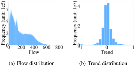
To tackle the underfitting problem during prediction making, we design a novel method named First-Order Gradient Supervision (FOGS). FOGS employs the first-order gradients, a.k.a. trends, rather than the exact flows to train the prediction model. Briefly speaking, at some moment, the trend is the relative temporal change of the flow from the previous moment. We show the distributions of flows and trends of the training set of the PEMS03 dataset 1 in Figure 1. As we can see, flows and trends have very different distributional properties. The flow distribution is irregularly shaped and widely spread, while the trend distribution is well concentrated. This is consistent with our intuition that the human activities follow some regular patterns in general, although the exact flows may differ from one day to another. Therefore, we argue that trends will provide more supervision for flow prediction. FOGS aims to make wise use of such supervision from trends.
In summary, we make the following contributions to traffic flow prediction:
1 This dataset contains traffic flow data recorded by 358 sensors from 1 Sept 2018 to 30 Nov 2018 in California. See Section 6 for further details.
- We propose a novel graph embedding approach to learn a data representation for each sensor. Comparing to existing solutions, our data representation better reflects both temporal and spatial correlations between sensors.
- We reveal the importance of trends in flow prediction. We propose a novel method, FOGS, which can make wise use of the supervision information provided by trends for accurate flow prediction.
- We conduct extensive experiments on four real-world datasets to test the performance of FOGS. The results show that FOGS significantly outperforms the existing solutions in terms of accuracy.
2 RelatedWork
Recently, graph convolution methods have been widely used to model the spatiotemporal correlations in traffic network data. DCRNN [Li et al., 2018] employs bi-directional random walks to characterize the diffusion process regarding spatial relationships. It combines gated recurrent units (GRU) with diffusion convolution, and then proposes an encoderdecoder model for temporal correlations. STGCN [Yu et al., 2018] utilizes convolutional structures on spatial and temporal domain to extract spatiotemporal features simultaneously. ASTGCN [Guo et al., 2019] proposes to utilize spatial and temporal attention mechanism to learn spatial and temporal correlations, respectively. STSGCN [Song et al., 2020] employs spatiotemporal synchronous graph convolutional module to directly capture the localized spatiotemporal correlations. STFGNN [Li and Zhu, 2021] uses the dynamic time warping (DTW) algorithm to construct a temporal graph and merges it with a given spatial graph into a novel spatiotemporal fusion graph. As mentioned in Section 1, the graphs used by these methods are manually built, thus human experience may affect the prediction performance.
3 Preliminaries and Problem Statement
In this section, we formally introduce the traffic flow prediction problem with necessary definitions and preliminaries.
3.1 Definitions
Road network. A road network is an undirected graph R = (V, Eroad), where V and Eroad are the sets of sensors and the road segments between sensors, respectively. The road network R indicates the spatial relationship between sensors, which remains static over time.
Traffic flow & graph signal. Given a road network R = (V, Eroad) and a sequence of T consecutive time intervals, the observed graph signal on R during the t-th time interval is a nonnegative vector x(t) R ∈ R|V | , where the j-th element of x(t) R is the traffic flow observed by the j-th sensor during the t-th time interval.
3.2 Problem Statement
At time t, given a road network R and previous T graph signals x(t-T+1) R , · · · , x(t) R , the problem of traffic flow prediction is to find a function f to predict future K graph signals:
4 Spatiotemporal Correlation Learning
In this section, we present our method for learning the spatiotemporal correlations between sensors. The method works with a road network R, which reflects spatial correlations, and a temporal correlation graph C to generate a spatiotemporal representation for each sensor. By properly defining a neighborhood based on the learned representation, we obtain a graph depicting the spatiotemporal correlations between sensors, which can then be used for flow prediction.
4.1 Temporal Correlation Graph
Formally, the temporal correlation graph is C = (V,Etime), where V is the set of sensors, as in the road network R, and Etime represents temporal correlations between sensors. As explained in Section 1, when establishing Etime, we wish to make use of the temporal patterns at finer granularities.
To that end, we decompose a week into a sequence of equally-lengthed consecutive time slots, each corresponding to a certain time interval in a week (e.g., 0:00 to 0:05 A.M. on Wednesday). The length of each time slot is 1ω , where ω is the data collection frequency of sensors. Suppose that a week consists of Nω such time slots. Then, for each sensor v, we construct an Nω-dimensional feature vector, where the j-th element is the average of all the flows ever recorded by sensor v during the j-th time slot in a week.
Using such temporal feature vectors, (u, v) ∈ Etime if v is a k-nearest neighbor of u, where the neighborhood is decided by measures such as the Euclidean distance.
4.2 Objective Function
Given the road network R = (V, Eroad) and the temporal correlation graph C = (V,Etime), our next goal is to find an embedding function h : V → Rm that maps each sensor v ∈ V into an m-dimensional feature vector (i.e., embedding). The embedding function h(·) is expected to preserve the closeness between sensors in both R and C. In this sense, we essentially want to simultaneously learn an embedding function h and a correlation graph G = (V, E), where the spatiotemporal correlations between sensors are well reflected in E and well preserved by h.
To implement the learning, we use the skip-gram method [Mikolov et al., 2013] to capture the "neighborhood" properties. The learning objective used in our work is
Here, NS(v) ⊆ V is the "neighbors" of sensor v, which, in our context, refers to all the sensors reachable from v under some sampling strategy S. Pr (NS(v)|h(v)) is the probability of observing NS(v) given the embedding h(v). Assuming probabilistic independence, this probability can be calculated as
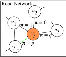
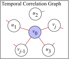
Figure 2: A simple illustration of our random walk sampling strategy. (a) The walk just traversed the edge (vj-1, vj) and stops at sensor vj now in the road network R. Then we want to choose the next sensor vj+1. (b) v0 is the starting sensor of the walk, and the traffic flow pattern of v0 is similar to that of vj-1, vj , u1, u3 but not to u2 in the temporal correlation graph C.
where a common choice for Pr (u|h(v)) is
Consequently, the objective becomes
4.3 Optimizing the Objective Function
Figure 2 illustrates our random walk process. Clearly, the objective function of Eq. 2 is largely affected by the neighborhood function NS(·), which is in turn determined by the sampling strategy S. Direct computation of the objective function may be prohibitive in practice, as we need to traverse V , the entire set of sensors, to compute the sum Ψ(v) during the training process. Such a traversal should be done every time the embedding function h(·) is updated, since there is no easy way to reuse the results.
The problem can be solved using random walks and negative sampling [Grover and Leskovec, 2016; Han et al., 2021]. Starting from a source sensor v0 ∈ V , a random walk of length L generates a path τ = ⟨v0, v1, · · · , vL⟩. With a predefined threshold ∆ (∆ ≪ L), we may obtain a set of neighbors of vj from the path τ ,
where j = 0, 1, · · · ,L. Essentially, Nτ(vj) is a sample of NS(vj), the sensors in which are intuitively closer to vj than the others are. Such discrimination can then be fed into optimization algorithms such as stochastic gradient descent (SGD) to find the optimal embedding h.
Conventional graph embedding methods generate random walks based on the topological structure to find the set of neighbors, which makes no use of the temporal correlations. In this work, we propose a new sampling strategy S to take temporal correlations into account in randomwalks.
Let R = (V, Eroad) and C = (V, Etime) be the road network and the temporal correlation graph, respectively. Assume that a random walk starts from sensor v0 has so far generated a path τj = ⟨v0, · · · , vj-1, vj⟩. (Thus, the randomwalk is now at sensor vj .) The sampling strategy S decides the next sensor vj+1 to visit based on the probability:
Here, π(τj, vj+1) is a weight assigned to the (potential) edge (vj , vj+1):
where dR(vj+1) is the shortest path distance between vj+1 and vj-1 ∈ τj in the road network R.
There are three choices for the next sensor vj+1: (i) sensor vj-1, (ii) sensor u1 near vj-1, and (iii) sensor u2 or u3 away from vj-1. Therefore, dR(vj+1) must be 0, 1, or 2. In this way, we could guarantee that the traffic flow patterns of all the sensors in a random walk is similar to that of the source sensor v0. Meanwhile, the proposed sampling method can retain the topology structure of the road network as well.
5 First-Order Gradient Supervision
In this section, we present FOGS, our novel traffic flow supervision method.
5.1 First-Order Gradient
Existing studies typically utilize the exact traffic flows to train their models and then predict the future flows in the network. However, we argue that there are many external factors affecting the traffic flow at a particular sensor, such as geographical location, facilities in the surrounding area, etc. As shown in Figure 1(a), the distribution of traffic flows is irregularly shaped, which is difficult to fit with limited amount of training data. Nonetheless, from Figure 1(b), we observe that the distribution of trends is concentrated.
Based on such observation, we propose a novel approach, namely FOGS, which focuses on trends instead of traffic flows. Recall that traffic flow prediction is to find a function f to predict future K graph signals based on the previous T ones. Therefore, from any data available, we have training samples of the form X → Y , where
is the matrix of T consecutive graph signals and
is the matrix of the next K ones right after xT , i.e., yt = xT+t for t = 1, 2, · · · ,K.
For the j-th sensor vj ∈ V , we define the trend of the traffic flow at vj at time T + t, denoted zjt, as follows:
The trend zjt is the relative change of yjt over xjT , the last observed flow by sensor vj. In occasional cases, xjT = 0. Then, we look backwards in time, scanning xj(T-1), xj(T-2), · · · , xj1 in order for the first nonzero value and use it as the reference for the relative change. 2 Eventually, given a training sample X → Y , we obtain a trend matrix Z of the same shape of Y .
5.2 Spatiotemporal Correlation Graph
Since we have learned an embedding function h(·) over the sensors V , which well preserves both the spatial and temporal correlations, we are now ready to construct a learning-based spatiotemporal correlation graph G.
To do this, we first compute a spatiotemporal correlation matrix M ∈ [0, 1]|V |×|V | between each pair of sensors. Specifically, the (i, j)-th entry of M is defined as
2 There is still chance that xjt ≡ 0 for every t = 1, 2, · · · , T. In this case, we replace xjt with first nonzero flow average recorded by sensor j in same way. However, the flow averages could still be zero, we choose to replace xjt with constant σ = 5.
Based on M, we may calculate a k-nearest neighbor set for each sensor vj, using, for example, the Euclidean distance. Then, we have
Finally, by normalizing the matrix G, we obtain the learned spatiotemporal correlation graph G:
where D = diag (G) denotes the out-degree diagonal matrix derived from G.
5.3 Model Framework
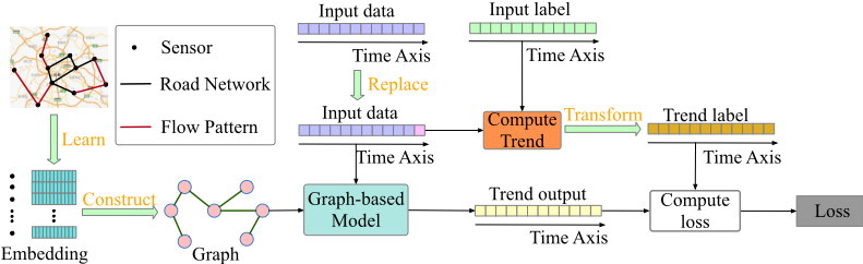
Figure 3 shows the FOGS framework. The replaced input data X and the spatiotemporal correlation graph G are fed into the graph-based model g to obtain the prediction output, i.e., the trend matrix:
where g denotes a prediction model such as STFGNN.
We choose MAE loss as the loss function, which is defined as follows:
During evaluation phase, we convert the predicted trends ˆZ ∈ R|V |×K back into corresponding traffic flows ˆ Y :
where XT is the |V | ×K matrix with the traffic signal xT duplicated K times, and ⊙ is the Hadamard product.
6 Experiments
In this section, extensive experiments are conducted to show the effectiveness of our approach. We first introduce the datasets and the baseline methods. Then, we introduce the experimental results and analyses by comparing with the baselines. Finally, we conduct ablation experiment to show the effect of some components in our framework.
6.1 Datasets
We conduct experiments on four real-world datasets from [Song et al., 2020]: PEMS03, PEMS04, PEMS07, and PEMS08. The data are extracted from Caltrans Performance Measurement System (PeMS) [Chen et al., 2001] in four different districts in California. The raw data are aggregated into 5-minute time intervals, thus there are 12 points in the traffic data per hour. Each sensor in PEMS04 and PEMS08 has three traffic-related data: flow, occupancy, and speed. In this paper, we use the flow data and ignore the rest. Table 1 shows the statistics of the four datasets used in our experiments.
Same as what previous studies [Song et al., 2020; Li and Zhu, 2021] do, we map each sensor v into real road networks to construct the the road network of sensors, i.e., R in Section 3. In addition, we utilize Z-score normalization to standardize the input data.
| Dataset | #Days | #Sensors | #Edges | #Data |
|---|---|---|---|---|
| PEMS03 | 91 | 358 | 547 | 26208 |
| PEMS04 | 59 | 307 | 340 | 16992 |
| PEMS07 | 98 | 883 | 866 | 28224 |
| PEMS08 | 62 | 170 | 295 | 17856 |
6.2 Settings
We split these four datasets with ratio 7 : 1 : 2 into training, validation, and test sets. We use the flows of one hour to predict the ones in the next hour. That is, we set T = K = 12 in our experiments, using 12 continuous graph signals to predict the next 12 ones. The parameters p and q in our random walk strategy, as introduced in Section 4, are both set to 1. When constructing the temporal correlation graph C (Section 4) and the final spatiotemporal correlation graph G (Section 5), we consider k = 10 nearest neighbors for each sensor. Moreover, we set the dimension of sensor embeddings to 128 , the random walk length L to 25, and the window threshold ∆ to 10. Our implementation is available in Pytorch 3 .
6.3 Baselines
We consider the following five state-of-the-art methods as the baselines in the experiments.
- ASTGCN [Guo et al., 2019]: Attention Based Spatial Temporal Graph Convolutional Networks, which models spatial and temporal correlations with spatial and temporal attention mechanisms. To conduct a fair comparison, only the recent components are used to model the periodicity of the traffic data.
- DCRNN [Li et al., 2018]: Diffusion Convolutional Recurrent Neural Network, which incorporates encoderdecoder model with diffusion graph convolution.
- STGCN [Yu et al., 2018]: Spatial-Temporal Graph Convolutional Networks, which only utilizes convolutional structures on spatial and temporal domains to extract spatiotemporal features simultaneously.
- STSGCN [Song et al., 2020]: Spatial-Temporal Synchronous Graph Convolutional Networks, which constructs a localized spatiotemporal graph to capture spatiotemporal correlations simultaneously.
- STFGNN [Li and Zhu, 2021]: Spatial-Temporal Fusion Graph Neural Networks, which designs a spatiotemporal fusion graph. A fusion graph neural module and a gated convolution module are combined to model spatiotemporal correlations.
For our method FOGS, we choose STFGNN as the base prediction model.
6.4 Results and Analysis
The experiment results on the four public datasets are shown in Table 2. Based on these results, we have the following observations and corresponding analysis:
3 https://github.com/kevin-xuan/FOGS
| Datasets | Metric | ASTGCN | DCRNN | STGCN | STSGCN | STFGNN | FOGS (ours) |
|---|---|---|---|---|---|---|---|
| PEMS03 | MAE MAPE(%) RMSE | 18.05 17.02 30.13 | 17.86 18.30 29.74 | 17.52 17.08 30.23 | 17.17 16.17 28.58 | 16.80 16.23 28.44 | 15.06 14.11 24.25 |
| PEMS04 | MAE MAPE(%) RMSE | 21.85 14.11 34.54 | 23.54 17.18 36.25 | 22.72 14.56 35.56 | 20.98 13.73 33.58 | 19.85 12.99 31.89 | 19.35 12.71 31.33 |
| PEMS07 | MAE MAPE(%) RMSE | 25.22 11.41 38.83 | 23.87 10.50 37.27 | 24.58 10.65 37.51 | 23.39 9.83 37.79 | 21.51 9.02 35.67 | 20.62 8.58 33.96 |
| PEMS08 | MAE MAPE(%) RMSE | 18.70 11.64 28.66 | 18.41 12.17 28.28 | 18.14 11.38 27.97 | 16.35 10.54 25.64 | 16.75 10.58 26.35 | 14.92 9.42 24.09 |
- Our proposed methods significantly outperform all other state-of-the-art baselines under all metrics on all datasets. Specifically, FOGS outperforms ASTGCN, DCRNN, STGCN, STSGCN and STFGNN with ratios 19.52%, 18.46%, 19.78%, 15.15%, and 14.73%, respectively under the RMSE metric on PEMS03 dataset. This shows the superiority of our framework to some extent.
- Comparing STFGNN and our method FOGS, we can find that our proposed methods greatly improve the performance. The reason might be that the spatiotemporal correlation graph G used in our method is learned, instead of manually constructed, which could better capture the spatiotemporal information. Moreover, it also demonstrates that training models with trends instead of traffic flows could enhance the models performance.
- Comparing the performance improvement on the PEMS04 ans PEMS07 datasets, we could see that FOGS performs better on the PEMS03 and PEMS08 datasets. The reason might be that the road network is more sparse on PEMS04 and PEMS07 datasets, which leads to the inaccuracy of the learned graph G. Moreover, a higher rate of missing traffic data will also result in poor model performance.
6.5 Ablation Experiment
There are two main components in our framework: (i) the learned graph, and (ii) the trend supervision. To show the effects of these components, we conduct ablation experiments on FOGS, of which the results are shown in Table 3.
From Table 3, we may have the following conclusions and analyses:
- We can find that our learned graph could improve the model performance. Because the sensor embedding learned through the random walk algorithm can not only reflect the topology of the spatial network, but also reflect historic traffic flow patterns. The combination of them allows the learned graph to make effective use of the side information.
- We could notice that training STFGNN model with trend could improve model performance on all datasets. Be-
| Datasets | Metric | Baseline | Graph | Trend |
|---|---|---|---|---|
| PEMS03 | MAE MAPE(%) RMSE | 16.80 16.23 28.44 | 15.53 14.82 27.24 | 15.06 14.11 24.25 |
| PEMS04 | MAE MAPE(%) RMSE | 19.85 12.99 31.89 | 19.48 12.81 31.56 | 19.34 12.71 31.20 |
| PEMS07 | MAE MAPE(%) RMSE | 21.51 9.02 35.67 | 20.88 8.80 34.40 | 20.62 8.58 33.96 |
| PEMS08 | MAE MAPE(%) RMSE | 16.75 10.58 26.35 | 15.47 9.95 24.78 | 14.92 9.42 24.09 |
cause trends tend to be consistent and concentrated, training model with trends can significantly enhance the model performance.
7 Conclusion
In this paper, we propose a novel learning-based approach to learn a graph that could make effective use of the information in spatio-temporal data. Embedding of every sensor is learned by our sampling method, which could capture the topology structure of the road network and historic traffic flow patterns. The graph is constructed by the cosine values between embeddings of sensors with k-nearest neighbors. Moreover, a novel supervised method, FOGS is presented to enhance model performance, which uses trend rather than specific flow to train models. We conduct extensive experiments and analysis on four public datasets, which show that our proposed approaches significantly outperform the existing baselines.
Acknowledgements
This work was supported by the NSFC (U2001212, 62032001, and 61932004).
@inproceedings{ijcai2022p545,
  title     = {FOGS: First-Order Gradient Supervision with Learning-based Graph for Traffic Flow Forecasting},
  author    = {Rao, Xuan and Wang, Hao and Zhang, Liang and Li, Jing and Shang, Shuo and Han, Peng},
  booktitle = {Proceedings of the Thirty-First International Joint Conference on
               Artificial Intelligence, {IJCAI-22}},
  publisher = {International Joint Conferences on Artificial Intelligence Organization},
  editor    = {Luc De Raedt},
  pages     = {3926--3932},
  year      = {2022},
  month     = {7},
  note      = {Main Track},
  doi       = {10.24963/ijcai.2022/545},
  url       = {https://doi.org/10.24963/ijcai.2022/545},
}
TY - CPAPER TI - FOGS: First-Order Gradient Supervision with Learning-based Graph for Traffic Flow Forecasting AU - Rao, Xuan AU - Wang, Hao AU - Zhang, Liang AU - Li, Jing AU - Shang, Shuo AU - Han, Peng T2 - Proceedings of the Thirty-First International Joint Conference on Artificial Intelligence, IJCAI-22 PB - International Joint Conferences on Artificial Intelligence Organization PY - 2022 SP - 3926 EP - 3932 DO - 10.24963/ijcai.2022/545 UR - https://doi.org/10.24963/ijcai.2022/545 ER -Copied
Machine-readable versions of this paper, for tools and AI agents:





