
Learning and Exploiting Progress States in Greedy Best-First Search
Proceedings of the Thirty-First International Joint Conference on Artificial Intelligence. Main Track. Pages 4740-4746.
https://doi.org/10.24963/ijcai.2022/657
Keywords
- Planning and Scheduling: Learning in Planning and Scheduling
- Planning and Scheduling: Search in Planning and Scheduling
- Search: Search and Machine Learning
- Search: Heuristic Search
Abstract
Previous work introduced the concept of progress
states. After expanding a progress state, a greedy
best-first search (GBFS) will only expand states
with lower heuristic values. Current methods can
identify progress states only for a single task and
only after a solution for the task has been found.
We introduce a novel approach that learns a description
logic formula characterizing all progress
states in a classical planning domain. Using the
learned formulas in a GBFS to break ties in favor
of progress states often significantly reduces the
search effort.
- [Baader et al., 2003] Franz Baader, Diego Calvanese, Deb- orah L. McGuinness, Daniele Nardi, and Peter F. Patel- Schneider, editors. The Description Logic Handbook: Theory, Implementation and Applications. Cambridge University Press, 2003.
- [Breiman et al., 1984] Leo Breiman, J. H. Friedman, R. A. Olshen, and C. J. Stone. Classification and Regression Trees. Wadsworth, 1984.
- [Dechter and Pearl, 1985] Rina Dechter and Judea Pearl. Generalized best-first search strategies and the optimality of A * . JACM, 32(3):505-536, 1985.
- [Doran and Michie, 1966] James E. Doran and Donald Michie. Experiments with the graph traverser program. Proceedings of the Royal Society A, 294:235-259, 1966.
- [Drexler et al., 2022] Dominik Drexler, Guillem Francès, and Jendrik Seipp. Description logics state features for planning (DLPlan). https://doi.org/10.5281/zenodo. 5826139, 2022. DOI
- [Ferber et al., 2022] Patrick Ferber, Liat Cohen, Jendrik Seipp, and Thomas Keller. Code, data, and supplement for the IJCAI 2022 paper "Learning and Exploiting Progress States in Greedy Best-First Search". https://doi.org/10. 5281/zenodo.6496715, 2022. DOI
- [Fikes and Nilsson, 1971] Richard E. Fikes and Nils J. Nils- son. STRIPS: A new approach to the application of theo- rem proving to problem solving. AIJ, 2:189-208, 1971. IJCAI
- [Francès et al., 2021a] Guillem Francès, Blai Bonet, and Hector Geffner. Learning general planning policies from small examples without supervision. In Proc. AAAI 2021, pages 11801-11808, 2021.
- [Francès et al., 2021b] Guillem Francès, Blai Bonet, and Hector Geffner. Learning general policies from small ex- amples without supervision. arXiv:2101.00692 [cs.AI], 2021.
- [Helmert and Röger, 2008] Malte Helmert and Gabriele Röger. How good is almost perfect? In Proc. AAAI 2008, pages 944-949, 2008.
- [Helmert, 2006] Malte Helmert. The Fast Downward plan- ning system. JAIR, 26:191-246, 2006.
- [Heusner et al., 2017] Manuel Heusner, Thomas Keller, and Malte Helmert. Understanding the search behaviour of greedy best-first search. In Proc. SoCS 2017, pages 47- 55, 2017.
- [Heusner et al., 2018] Manuel Heusner, Thomas Keller, and Malte Helmert. Best-case and worst-case behavior of greedy best-first search. In Proc. IJCAI 2018, pages 1463- 1470, 2018. IJCAI
- [Hoffmann and Nebel, 2001] Jörg Hoffmann and Bernhard Nebel. The FF planning system: Fast plan generation through heuristic search. JAIR, 14:253-302, 2001.
- [Holte, 2010] Robert C. Holte. Common misconceptions concerning heuristic search. In Proc. SoCS 2010, pages 46-51, 2010.
- [Imai and Fukunaga, 2015] Tatsuya Imai and Alex Fuku- naga. On a practical, integer-linear programming model for delete-free tasks and its use as a heuristic for cost- optimal planning. JAIR, 54:631-677, 2015.
- [Korf et al., 2001] Richard E. Korf, Michael Reid, and Ste- fan Edelkamp. Time complexity of iterative-deepening A * . AIJ, 129:199-218, 2001.
- [Martelli, 1977] Alberto Martelli. On the complexity of ad- missible search algorithms. AIJ, 8:1-13, 1977.
- [McDermott et al., 1998] Drew McDermott, Malik Ghallab, Adele Howe, Craig Knoblock, Ashwin Ram, Manuela Veloso, Daniel Weld, and David Wilkins. PDDL - The Planning Domain Definition Language -Version 1.2. Technical Report CVC TR-98-003/DCS TR-1165, Yale Center for Computational Vision and Control, Yale Uni- versity, 1998.
- [Meurer et al., 2017] Aaron Meurer, Christopher Smith, Ma- teusz Paprocki, Ondřej Čertík, Sergey Kirpichev, Matthew Rocklin, AMiT Kumar, Sergiu Ivanov, Jason Moore, Sar- taj Singh, Thilina Rathnayake, Sean Vig, Brian Granger, Richard Muller, Francesco Bonazzi, Harsh Gupta, Shivam Vats, Fredrik Johansson, Fabian Pedregosa, Matthew Curry, Andy Terrel, Štěpán Roučka, Ashutosh Saboo, Isuru Fernando, Sumith Kulal, Robert Cimrman, and An- thony Scopatz. SymPy: symbolic computing in Python. PeerJ Computer Science, 3:e103, 2017.
- [Pearl, 1984] Judea Pearl. Heuristics: Intelligent Search Strategies for Computer Problem Solving. Addison- Wesley, 1984.
- [Pedregosa et al., 2011] Fabian Pedregosa, Gaël Varoquaux, Alexandre Gramfort, Vincent Michel, Bertrand Thirion, Olivier Grisel, Mathieu Blondel, Peter Prettenhofer, Ron Weiss, Vincent Dubourg, Jake Vanderplas, Alexandre Pas- sos, David Cournapeau, Matthieu Brucher, Matthieu Per- rot, and Édouard Duchesnay. Scikit-learn: Machine learn- ing in Python. Journal of Machine Learning Research, 12:2825-2830, 2011.
- [Seipp et al., 2017] Jendrik Seipp, Florian Pommerening, Silvan Sievers, and Malte Helmert. Downward Lab. https: //doi.org/10.5281/zenodo.790461, 2017. DOI
- [Seipp et al., 2022] Jendrik Seipp, Álvaro Torralba, and Jörg Hoffmann. PDDL generators. https://doi.org/10.5281/ zenodo.6382173, 2022. DOI
- [Ståhlberg et al., 2021] Simon Ståhlberg, Guillem Francès, and Jendrik Seipp. Learning generalized unsolvability heuristics for classical planning. In Proc. IJCAI 2021, pages 4175-4181, 2021. IJCAI
- [Torralba et al., 2021] Álvaro Torralba, Jendrik Seipp, and Silvan Sievers. Automatic instance generation for classical planning. In Proc. ICAPS 2021, pages 376-384, 2021.
- [Wilt and Ruml, 2014] Christopher Wilt and Wheeler Ruml. Speedy versus greedy search. In Proc. SoCS 2014, pages 184-192, 2014.
- [Wilt and Ruml, 2015] Christopher Wilt and Wheeler Ruml. Building a heuristic for greedy search. In Proc. SoCS 2015, pages 131-139, 2015.
- [Wilt and Ruml, 2016] Christopher Wilt and Wheeler Ruml. Effective heuristics for suboptimal best-first search. JAIR, 57:273-306, 2016.
References were extracted automatically from the PDF and may contain errors.
Full text extracted automatically from the PDF; figures, tables and equations may differ. The PDF is the version of record.
1 Introduction
Theoretical properties of optimal state-space search algorithms like A* or IDA* have been extensively studied and are comparatively well understood [Martelli, 1977; Pearl, 1984; Dechter and Pearl, 1985; Korf et al., 2001; Helmert and R¨oger, 2008; Holte, 2010]. A corresponding theory for suboptimal search algorithms like greedy best-first search (GBFS) [Doran and Michie, 1966] has received growing attention only in the last couple of years [Wilt and Ruml, 2014; Wilt and Ruml, 2015; Wilt and Ruml, 2016; Heusner et al., 2017; Heusner et al., 2018].
The main insight of Heusner et al. [2017] is that every run of a GBFS can be partitioned into different episodes defined by so-called high-water mark benches, and the statespace topology can be partitioned in the same way. All states s on a bench share the same high-water mark value, which is the largest heuristic value that needs to be considered to reach a goal state from s. Progress states are states that must be expanded to reach the next high-water mark bench. Exploiting knowledge of high-water mark benches or progress states during search gives rise to many applications. The only known algorithm that computes high-water mark benches does so a posteriori, i.e., it computes the benches of a problem, after a plan was found [Heusner et al., 2018]. At this point, the high-water mark information is futile.
Inspired by St˚ahlberg et al. [2021], who successfully learn to characterize unsolvable states using description logic [Baader et al., 2003], we present an approach that learns to characterize progress states. First, we verify for the GRIPPER and MICONIC planning domains that the set of progress states for the perfect delete-relaxed heuristic h+ [Hoffmann and Nebel, 2001; Imai and Fukunaga, 2015] can be compactly represented with a description logic formula. Then, we present a method to learn such formulas automatically for any path-independent heuristic.
Our pipeline works as follows: for a given domain and heuristic, we fully expand the reachable state spaces of several small tasks and annotate all states with their heuristic value. Based on the heuristic values, we determine for each state whether it is a progress state. Next, we compute a set of description logic features and evaluate each of them on a subset of states. Then, we adapt a decision tree [Breiman et al., 1984] learning algorithm to learn simple formulas over the description logic features in disjunctive normal form (DNF) which predict whether a state is a progress state. Finally, we show a first use case for the learned progress state classifier: we use our formulas to break ties in a greedy best-first search.
We evaluate our method using the h+ and hFF heuristics [Hoffmann and Nebel, 2001] and show that our approach successfully learns useful formulas to identify progress states. We observe a trade-off between the quality of the formulas and the time to evaluate them. Most importantly, we show that exploiting progress states is beneficial: it significantly reduces the number of expansions required to find a plan.
2 Background
We first introduce the used planning formalism and provide a short introduction to description logic. Then, we formally define progress states and explain how decision trees work.
2.1 Classical Planning
Throughout this paper, we work with STRIPS tasks [Fikes and Nilsson, 1971] defined in the Planning Domain Description Language (PDDL) [McDermott et al., 1998]. A task Π is a tuple 〈O, P, A, sI , γ〉, where O is a set of objects and P is a set of first-order predicates. A predicate p ∈ P with arity k grounded to p(o1, o2, . . . , ok) with oi ∈ O is called a fact. Let F be the set of all facts. Then any s ⊆ F is called a state and the set of all states S is called a state space. sI ∈ S is the initial state and γ ⊆ F is the goal condition. All states s ⊇ γ are goal states. A is a set of action schemas that can be grounded using O. We call grounded action schemas actions.
An action a is a tuple 〈pre, add, del〉 with pre, add, del ⊆ F and is associated with a cost cost(a) ∈ R+0 . Action a is applicable in state s if pre ⊆ s. Applying a in s, written as sJaK, leads to the successor state (s \ del) ∪ add. An action sequence π = 〈a1, a2, . . . , an〉 is applicable in state s if every action ai is applicable in the state sJa1KJa2K . . . Jai-1K. The cost of an action sequence is the summed-up cost of its actions. A state s′ is reachable from s if there is an applicable action sequence starting in s and ending in s′ . The reachable state space SR ⊆ S is the set of all states reachable from sI . An applicable action sequence starting in state s and ending in a goal state is called an s-plan. The objective in classical planning is to find an sI-plan, i.e., a plan for the given task.
2.2 Description Logic
Description logic (DL) is a family of knowledge representation formalisms [Baader et al., 2003] which uses the notions of concepts, classes of objects that share some property, and roles, relations between these objects. Interpreting concepts and roles for a planning state yields a denotation, i.e., a set of objects O ⊆ O for a concept, and a set of object pairs {〈o1, o2〉, 〈o3, o4〉, . . .} ⊆ O × O for a role.
Concepts and roles are recursively defined and interpreted for a state s ∈ S. At its base are the universal concept ⊤ and the bottom concept ⊥ with semantics
as well as primitive concepts and roles. A primitive concept Cp,i for a k-ary predicate p ∈ P and its i-th argument is interpreted in s as
Accordingly, a primitive role Rp,i,j for a k-ary predicate p ∈ P and its i-th and j-th arguments is interpreted as
in s. Let X and X′ be two concepts resp. two roles. They can be combined to form new concepts and roles via grammar rules. Examples are negation, union, and intersection which are interpreted in a state s as
We use the same grammar as Franc`es et al. [2021a]. For details, we refer to their extended paper [Franc`es et al., 2021b].
We use two functions to convert denotations to integers. For a concept or role X, |X(s)| is the size of the set X(s). The concept distance cd between concepts C1 and C2 over role R is the smallest n ∈ N0 with x0 ∈ C1(s), xn ∈ C2(s), and all (xi, xi+1) ∈ R(s).
The complexity K(X) of the universal concept, the bottom concept, any primitive concept, and any primitive role is 1. The complexity of composed concepts and roles is defined as
2.3 Progress States
Let Π be a planning problem with a state s. A heuristic h : S → R+0 ∪ {∞} estimates the cost of an optimal splan. Let P be the set of all acyclic s-plans. The high-water mark of s is
Heusner et al. [2018] define a state s as progress state iff its high-water mark is larger than the high-water mark of at least one of its successor states. Counter-intuitively, this definition excludes goal states for goal-aware heuristics. We therefore adapt the definition: a state s is a progress state iff γ ⊆ s or h(s) > mins′∈succ(s) hwm(s′ ), where succ(s) is the set of all successor states of s and γ is the goal condition.
2.4 Decision Trees
A binary decision tree is a machine learning model with a binary tree structure [Breiman et al., 1984]. Let C be a set of classes and let F be a list of features. A decision tree assigns a class c ∈ C to a vector v ∈ RF . Each internal tree node i is associated with a feature f(i) ∈ {1, . . . , F} and a threshold τ(i) ∈ R. Each leaf node l is associated with a class class(l) ∈ C. To assign a class to an input vector v, the decision tree is traversed from the root node to a leaf node. At every internal node i, if v[f(i)] ≤ τ(i), then the traversal continues at the first child node, otherwise it continues at the second one. Once a leaf node l is reached, the input is labeled as class(l).
Decision trees are greedily constructed given some training data 〈D,L〉 with the feature matrix D ∈ RM×F and the label vector L ∈ CM where M is the number of training samples. Each node n is associated with a non-exclusive submatrix Dn ∈ RM′×F and Ln ∈ RM′ . The root node is associated with the whole training data D and L and is initially a leaf node. A leaf node l is associated with the most frequent class in Ll. During training, the algorithm chooses a leaf node l and searches through combinations of features f ′ and thresholds τ ′ . f ′ and τ ′ are used to group the data points 〈Dl[i],Ll[i]〉 for i ∈ {1, ...,M ′ } into two sets using the test Dl[i][f ′ ] ≤ τ ′ . The quality of the groups is evaluated using a metric (e.g., Gini impurity [Breiman et al., 1984]). The leaf is associated with the combination of the best split (f(l) = f ′ and τ(l) = τ ′ ) and two child leaves are added to it, one per split data set. This transforms l into an internal node.
The algorithm continues until all leaves contain only labels from the same class or a maximum tree depth is reached.
3 Handcrafted Formulas
An important first step is to verify that our design space, DNF formulas over description logic features, is expressive enough to compactly characterize progress states. Therefore, we manually create description logic formulas for two standard planning domains, GRIPPER and MICONIC. In contrast to the experiment section, we only consider h+ here, because it is easier to reason about than hFF . The presented formulas have been verified empirically on all training and validation instances (see below). We slightly simplify the description logic notation here by using constant objects directly and by defining ps(·) = Cp,0(s) and ps(·, o) = {o′ | 〈o′ , o〉 ∈ Rp,0,1(s)} for predicate p, state s, concept C and role R.
3.1 GRIPPER
An instance in the GRIPPER domain features a single robot with two grippers. The robot can move between two rooms roomA and roomB, and the goal is to move all balls from roomA to roomB. A GRIPPER state s is a progress state iff
The formula describes three types of progress states: (i) there are no balls in roomA, (ii) the robot is in roomA and has a free gripper or (iii) the robot is in roomB and carries at least one ball. In case (i), we are either in a goal state or moving to roomB makes progress; in case (ii), picking up a ball makes progress (unless case (i) holds); and in case (iii), dropping a ball makes progress.
3.2 MICONIC
In MICONIC, there is an elevator that operates in a fully connected graph, bringing passengers from an origin floor to a destination floor. Let fs be the floor for which lift-ats (fs) holds in state s. A MICONIC state s is a progress state iff
The formula describes three types of progress states: (i) the first line describes states where the elevator is at a floor that is the origin of at least one passenger that is not boarded and has not been served yet; (ii) the second line describes states where the elevator is at a floor that is the destination of at least one passenger that is boarded and has not been served yet; and (iii) the last line describes states where the elevator is at a floor that is not the destination of any passenger that is still waiting (i.e., not boarded and not served). In case (i), progress is made by letting a passenger board; in case (ii), progress is made by letting a passenger leave the elevator; and in case (iii), a goal state has been reached or progress is made by moving to another floor.
4 Learning to Characterize Progress States
In this section we describe our pipeline that labels states as progress states, calculates description logic features for them, and learns a DNF formula that identifies progress states.
4.1 Generating Labeled States
To label the states of a planning instance w.r.t. a heuristic h as progress or non-progress states, we first expand the reachable state space. This includes states reachable only on paths through goal states. For each state s, we track its predecessors pred(s), successors succ(s), and heuristic estimate h(s).
In a second iteration, we compute the high-water marks. Initially, we set hwm(g) = h(g) for all goal states g and regard hwm(s) as undefined for all other states s. We keep an open list of states ordered by high-water mark values that initially contains all goal states. Upon retrieving a state s from the open list, we insert all its predecessors p ∈ pred(s) with undefined high-water mark into the open list with a highwater mark value of hwm(p) = max(h(p), hwm(s)). The algorithm guarantees that a state is only inserted once into the open list, namely after its successor with lowest high-water mark value has been retrieved from the open list. When this process terminates, only unsolvable states have an undefined high-water mark, which we treat as ∞ from here on.
In a third iteration over all states, we label all states s that are goal states or that have at least one successor state with a lower high-water mark value (then hwm(s) > mins′∈succ(s) hwm(s′ )) as progress states. All remaining states (which includes those with hwm(s) = ∞) are nonprogress states. Note that it is possible to combine the second and third iteration into a single iteration, but considering two separate iterations simplifies the presentation.
4.2 Generating Description Logic Features
The next step of our pipeline takes as input a set of states labeled as "progress state" or "non-progress state", and a set of grammar rules that defines which features can be generated. The feature generation is an iterative process. In iteration i, only features of complexity i are generated. A new feature is pruned if it has the same denotation as a previously generated feature for all states. In the first iteration, all primitive concepts and roles, as well as the universal and bottom concepts are generated. In every succeeding iteration, the existing features are combined using the provided rules. The feature generation stops once all features up to a given complexity are generated or a time limit is reached.
As the decision tree learns formulas over Boolean features rather than sets of objects, we convert the denotation of each state feature to a Boolean value by first converting it to an integer i (unneeded for concept distance features) and then testing if i is greater than 0. Our feature language would be more expressive if we included comparisons between integer values derived from a feature or to other constants than 0. However, we observed that it is sufficient in most domains to check if a feature generates an empty set, and this restriction speeds up the feature generation significantly. After all features are generated, we iterate over the set of states and store for each state its label and the Boolean evaluation of every feature.
4.3 Learning DNF Formulas
We use the set of labeled states annotated with Boolean features to learn a DNF formula that characterizes progress states. There is no guarantee that our generated features perfectly separate progress from non-progress states. Our grammar might not be expressive enough or we might need a feature with a complexity that is infeasible to generate. Thus, we need a learning algorithm which allows imperfect separations. We decided to train decision trees.
Since our training data is already in an appropriate format (every state is represented by an equally-sized Boolean vector), we can apply a standard algorithm to obtain a decision tree. We do not limit the depth of the generated tree, so if it possible to separate the training data with the generated features, then the tree will separate them. After training the decision tree, we convert it to a DNF: we collect all paths in the tree which classify a state as progress state (e.g., 〈feature1 > 0 = ⊤, feature2 > 0 = ⊥〉). Each path becomes a clause in the DNF and each decision in the path becomes a literal. The path in the previous example implies a clause with the literals "feature1 > 0" and "feature2 = 0".
| Max. Complexity | # Features | ||||||
|---|---|---|---|---|---|---|---|
| Domain | 1. | 2. | 3. | 4. | 5. | Min | Max |
| BARMAN | 7 | 6 | 6 | 6 | 6 | 1218 | 2455 |
| BLOCKSWORLD | 10 | 10 | 10 | 10 | 10 | 15332 | 16611 |
| CHILDSNACK | 8 | 8 | 7 | 7 | 7 | 444 | 532 |
| DRIVERLOG | 9 | 8 | 8 | 7 | 7 | 892 | 1313 |
| FLOORTILE | 8 | 8 | 7 | 7 | 7 | 1644 | 3441 |
| GRIPPER | 12 | 12 | 9 | 9 | 9 | 422 | 1656 |
| MICONIC | 8 | 8 | 7 | 7 | 7 | 332 | 494 |
| VISITALL | 12 | 12 | 11 | 11 | 11 | 1692 | 2118 |
The automatically generated DNFs can be long and may contain redundancy, which makes them slow to evaluate and hard to interpret. We simplify the DNFs with SymPy [Meurer et al., 2017]. If several features separate the data equally well, we break ties first in favor of already used features and second in favor of lower complexity feature. This leads to a significantly lower number of distinct features in a formula which speeds up its evaluation and increases the probability that SymPy finds a simpler, logically equivalent formula.
5 Experiments
We explained above how we can use description logic to generate state features that generalize across all instances of a planning domain and how we can learn DNF formulas to predict whether a state is a progress or non-progress state. Now, we evaluate our pipeline on common planning domains and show that it learns useful formulas. To verify that the formulas learned important information, we use it as tie-breaker in a greedy best-first search (GBFS).
5.1 Setup
We evaluate our approach on the BARMAN, BLOCKSWORLD, CHILDSNACK, DRIVERLOG, FLOORTILE, GRIPPER, MICONIC, and VISITALL domains for the FF heuristic (hFF ) and the perfect delete-relaxed heuristic (h+) [Hoffmann and Nebel, 2001], using the formalization based on operator counting by Imai and Fukunaga [2015] for the latter. For each domain, we define a parameter space (e.g., a range for the number of balls in Gripper) and use it to generate small training and validation instances with PDDL task generators [Seipp et al., 2022]. As our test sets, i.e., for the GBFS runs with and without learned formulas, we use the union of Autoscale 21.11 tasks for optimal and satisficing planning [Torralba et al., 2021]. The test sets are are disjoint from and generally more challenging than our training and validation tasks. For each training and validation instance and each heuristic, we generate the labeled state space with a memory limit of 3.5 GiB and a time limit of 5 hours.
To generate the description logic features, we use the same concepts and roles as Franc`es et al. [2021a]. We use the size and the concept distance functions to convert the description logic features to integers. We observed that generating the features for a single state space can lead to features that are specific to that state space and to formulas that do not generalize to unseen tasks. Thus, we generate and evaluate 5 feature sets per domain, where the i-th feature set uses states from the first i training instances from that domain. We also observed that the feature generation often exceeds the available memory. As a solution, we select from each training instance a subset of up to 10000 progress and up to 10000 non-progress states. We impose no limit on the complexity of the generated features but instead limit the feature generation procedure to 24 hours and 3.5 GiB of memory.
The last step of our pipeline produces the DNF formulas. For each domain, we train a decision tree using each of the 5 generated feature sets. In some domains, one class (progress or non-progress states) heavily outnumbers the other class. Thus, we weight all samples such that both classes have the same impact on the final formula. Furthermore, since some training instances have state spaces of significantly different sizes, we additionally weight all samples to enforce that each instance has the same impact on the final formula. We evaluate all resulting formulas on the validation instances of their domain. Finally, for each domain we select the formula with the highest F1 score on the validation instances. In case of a tie, the formula with the better F1 score on the training instances and then the one trained on fewer state spaces is preferred. As the decision tree is a greedy learning algorithm, training is usually quick. We limit training of the DNF formulas to 10 minutes and their validation to 2 hours, both with a memory limit of 3.5 GiB.
Learning to identify progress states is an important contribution on its own. There are many ways in which a search can be improved if it knows which states are progress states or not. We will show that even imperfect formulas contain sufficient information to improve the search. We execute GBFS with hFF and h+ as baselines and then compare it to GBFS with the same heuristic that uses the progress state information to break ties if two states have the same heuristic value. For GRIPPER and MICONIC, we described perfect, handcrafted formulas above. To assess the quality of the learned formulas, we also compare them to their perfect counterparts.
We implemented the state space labeling and the final search in Fast Downward [Helmert, 2006]. To generate and evaluate the description logic features, we use the DLPlan library [Drexler et al., 2022], and we adapt scikit-learn [Pedregosa et al., 2011] to train the decision trees. To run our experiments, we use Downward Lab [Seipp et al., 2017]. All steps are executed on a single core of an Intel Xeon Silver CPU. Our benchmarks, code, experiment data, and supplemental results are available online [Ferber et al., 2022].
| Mean Validation F1 | First DNF | Best DNF | |||||||||
|---|---|---|---|---|---|---|---|---|---|---|---|
| Domain | 1. | 2. | 3. | 4. | 5. | K(F) | Clauses | Literals | K(F) | Clauses | Literals |
| BARMAN | 79 | 80 | 81 | 79 | 77 | 7 | 316 | 4059 | 6 | 1459 | 25189 |
| BLOCKSWORLD | 83 | - | - | - | - | 10 | 72 | 1009 | 10 | 72 | 1009 |
| CHILDSNACK | 70 | 65 | 73 | 81 | 72 | 8 | 28 | 240 | 7 | 116 | 1243 |
| DRIVERLOG | 81 | 81 | 89 | 85 | 85 | 9 | 95 | 829 | 8 | 1087 | 17270 |
| FLOORTILE | 75 | 85 | 85 | 85 | 88 | 8 | 10 | 91 | 7 | 65 | 926 |
| GRIPPER | 96 | 96 | 96 | 98 | 98 | 11 | 3 | 3 | 9 | 2 | 4 |
| MICONIC | 98 | 98 | 97 | 98 | 99 | 8 | 1 | 1 | 7 | 23 | 274 |
| VISITALL | 70 | 70 | 73 | 73 | 73 | 12 | 2413 | 42496 | 11 | 3744 | 74060 |
5.2 Results
We start our analysis by inspecting the output of the feature generation step. Table 1 shows for each domain the maximum complexity of features generated when using states from only one or up to five state spaces and the progress state labels for hFF . The results for h+ qualitatively look the same, so we only report them in the online supplement. We clearly see that using more state spaces causes the feature set to have lower complexity features. This is because more states cause more computational effort per feature. But more importantly, a more diverse training set helps to differentiate similar concepts and roles. As a result, fewer features are pruned and more features are created per complexity level. Thus, there is a trade-off between identifying the meaning of a feature more precisely and generating more complex features. Table 1 also shows that the number of generated features varies significantly between different domains. For example, we generate more than 16000 features in BLOCKSWORLD but fewer than 500 in MICONIC.
To compare different choices for the complexity trade-off, Table 2 shows the validation performance for DNF formulas trained on up to five state spaces. We see that training on a single state space already produces formulas with a good F1 score. Using more state spaces to generate the formula improves the performance only moderately. For BLOCKSWORLD, where a huge amount of features are generated (see Table 1), using more than one state space exhausts the memory.
Table 2 also shows that all DNFs (almost) always contain at least one of the most complex features available. This suggests that features of high complexity contain essential information. Comparing the number of clauses and literals between the first and best DNFs, it is apparent that the DNF trained on only a single state space requires significantly fewer clauses and literals - there are only two domains where formulas with more than 100 clauses are learned, and only one of them has more than 1000 clauses. On the other hand, the best DNF has more than 100 clauses in four domains, and three of those contain even more than 1000 clauses. A large DNF takes more time to evaluate and hence slows down search. Identifying the perfect trade-off between accuracy and evaluation speed remains future work.
| Domain | h+ | h+LOpt | h+L∗ |
|---|---|---|---|
| GRIPPER (17) | 137.68 | 57.03 | 57.03 |
| MICONIC (14) | 82.17 | 51.07 | 53.15 |
Below, we focus on the DNF formulas with the best F1 score, but results for other formulas can be found in the supplement. To indicate that hFF is enhanced by the best formula we write hFF L∗ and for h+ we write h+L∗ .
To show that it is indeed beneficial to characterize progress states, we use them to break ties in GBFS. Table 3 compares a standard GBFS with h+ against a GBFS with h+ which is enhanced by perfect progress state formulas. Using the perfect progress state formulas significantly reduces the required number of expansions, which indicates that it pays off to expand progress states as early as possible. We also see that the learned formula for GRIPPER is as good as the perfect formula. For MICONIC, the learned formula is slightly worse than the perfect one but still significantly better than performing a search without progress state information.
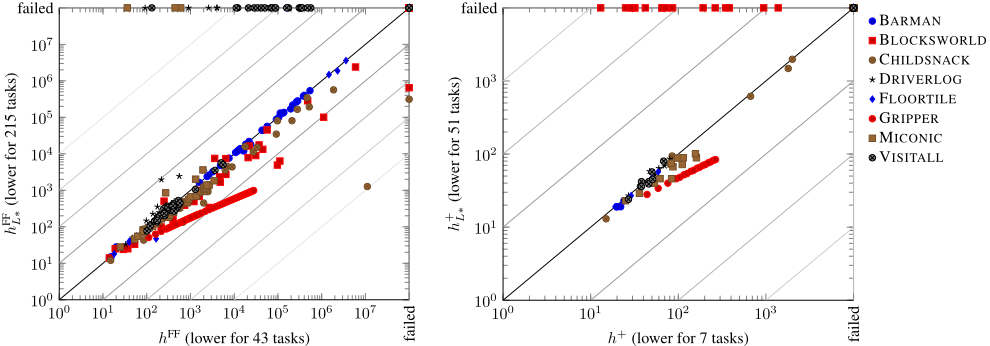
Finally, we evaluate the learned formulas for both h+ and hFF on all domains. Figure 1 compares the expansions required by GBFS with hFF (left) and h+ (right) to GBFS with the same heuristic and tie-breaking with the progress state information. Both plots show that exploiting the learned DNFs requires significantly fewer expansions in most planning instances. Plain hFF requires fewer expansions than our enhanced hFF L∗ in only 43 tasks, whereas the enhanced hFF L∗ requires fewer expansions in 215 tasks. The plain h+ heuristic requires fewer expansions in 7 tasks, whereas our enhanced h+L∗ requires fewer expansions in 51 tasks. This shows that our learned formulas successfully identify progress states and that exploiting progress states is a useful enhancement for a heuristic that guides GBFS.
Evaluating the progress state formulas in every state can be computationally expensive. Table 4 shows the geometric mean over the runtime on the commonly solved instances for our proof of concept implementation. For an expensive heuristic like h+, using the formulas does not only reduce the number of expansions, but also the runtime. However, in combination with a fast-to-evaluate heuristic like hFF , the time to evaluate a formula offsets the time saved due to the reduced number of expansions. Finding a sweet spot that optimizes the trade-off between formula complexity and accuracy will be the focus of future work.
| Domain | hFF | hFF L∗ | h+ | h+L∗ |
|---|---|---|---|---|
| BARMAN | 3.4 | 19.1 | 161 | 154 |
| BLOCKSWORLD | 0.3 | 0.5 | - | - |
| CHILDSNACK | 3.5 | 6.8 | 88 | 87 |
| DRIVERLOG | 0.1 | 3.2 | 244 | 252 |
| FLOORTILE | 0.4 | 0.9 | 11 | 11 |
| GRIPPER | 1.1 | 0.6 | 301 | 266 |
| MICONIC | 0.2 | 1.5 | 103 | 95 |
| VISITALL | 0.0 | 10.7 | 305 | 303 |
6 Conclusions
Heusner et al. [2017] showed that knowing which states in a GBFS are progress states bears great potential for improved algorithms. So far, however, this knowledge could only be computed a posteriori, making the information futile. We presented the first algorithm which learns a generalized model to identify progress states. The validation experiments verified that the formulas learned by our approach generalize across instances and that they are able to separate progress states from non-progress states with high accuracy. We furthermore showed that exploiting the learned information significantly decreases search effort, even with a simple baseline method that breaks ties in favor of progress states.
We believe this is only the first step in this direction of research. We observed that the selection of training instances and states from these instances has a huge impact on the quality of the learned formula, and so far we have not optimized the selection. It is furthermore unclear which feature complexity and which rules are necessary for a given domain. Even more importantly, our approach ignores the fact that a less accurate but faster-to-evaluate formula can be preferable in a search. Adapting the learning pipeline to produce formulas for specific use cases will be challenging future work.
Further ideas for future work include identifying not only progress states but also crater states and more sophisticated methods to exploit the learned knowledge, including methods that clear the open list when a progress state is encountered and search algorithms that actively avoid craters and search towards progress states.
Acknowledgments
This research was supported by TAILOR, a project funded by the EU Horizon 2020 research and innovation programme (grant agreement no. 952215). Patrick Ferber was partially supported by DFG grant 389792660 as part of TRR 248 (see https://perspicuous-computing.science). Liat Cohen was partially supported by the Eric and Wendy Schmidt Fund for Strategic Innovation and by the Council for Higher Education of Israel. Jendrik Seipp was partially supported by the Wallenberg AI, Autonomous Systems and Software Program (WASP) funded by the Knut and Alice Wallenberg Foundation, and Thomas Keller was partially supported by the European Research Council (ERC) under the European Union's Horizon 2020 research and innovation programme (grant agreement no. 817639).
@inproceedings{ijcai2022p657,
  title     = {Learning and Exploiting Progress States in Greedy Best-First Search},
  author    = {Ferber, Patrick and Cohen, Liat and Seipp, Jendrik and Keller, Thomas},
  booktitle = {Proceedings of the Thirty-First International Joint Conference on
               Artificial Intelligence, {IJCAI-22}},
  publisher = {International Joint Conferences on Artificial Intelligence Organization},
  editor    = {Luc De Raedt},
  pages     = {4740--4746},
  year      = {2022},
  month     = {7},
  note      = {Main Track},
  doi       = {10.24963/ijcai.2022/657},
  url       = {https://doi.org/10.24963/ijcai.2022/657},
}
TY - CPAPER TI - Learning and Exploiting Progress States in Greedy Best-First Search AU - Ferber, Patrick AU - Cohen, Liat AU - Seipp, Jendrik AU - Keller, Thomas T2 - Proceedings of the Thirty-First International Joint Conference on Artificial Intelligence, IJCAI-22 PB - International Joint Conferences on Artificial Intelligence Organization PY - 2022 SP - 4740 EP - 4746 DO - 10.24963/ijcai.2022/657 UR - https://doi.org/10.24963/ijcai.2022/657 ER -Copied
Machine-readable versions of this paper, for tools and AI agents:





