
Hidden 1-Counter Markov Models and How to Learn Them
Proceedings of the Thirty-First International Joint Conference on Artificial Intelligence. Main Track. Pages 4857-4863.
https://doi.org/10.24963/ijcai.2022/673
Keywords
- Machine Learning: Bayesian Learning
- Agent-based and Multi-agent Systems: Formal Verification, Validation and Synthesis
- Machine Learning: Time-series; Data Streams
- Uncertainty in AI: Graphical Models
- Uncertainty in AI: Bayesian Networks
Abstract
We introduce hidden 1-counter Markov models (H1MMs) as an attractive sweet spot between standard hidden Markov models (HMMs) and probabilistic context-free grammars (PCFGs). Both HMMs and PCFGs have a variety of applications, e.g., speech recognition, anomaly detection, and bioinformatics. PCFGs are more expressive than HMMs, e.g., they are more suited for studying protein folding or natural language processing. However, they suffer from slow parameter fitting, which is cubic in the observation sequence length. The same process for HMMs is just linear using the well-known forward-backward algorithm. We argue that by adding to each state of an HMM an integer counter, e.g., representing the number of clients waiting in a queue, brings its expressivity closer to PCFGs. At the same time, we show that parameter fitting for such a model is computationally inexpensive: it is bi-linear in the length of the observation sequence and the maximal counter value, which grows slower than the observation length. The resulting model of H1MMs allows us to combine the best of both worlds: more expressivity with faster parameter fitting.
- [Bahi-Jaber and Pontier, 2003] Narges Bahi-Jaber and Do- minique Pontier. Modeling transmission of directly trans- mitted infectious diseases using colored stochastic petri nets. Mathematical biosciences, 185(1):1-13, 2003.
- [Baker, 1979] James K Baker. Trainable grammars for speech recognition. The Journal of the Acoustical Soci- ety of America, 65(S1):S132-S132, 1979.
- [Baum and Petrie, 1966] Leonard E Baum and Ted Petrie. Statistical inference for probabilistic functions of finite state markov chains. The annals of mathematical statis- tics, 37(6):1554-1563, 1966.
- [Baum et al., 1970] Leonard E Baum, Ted Petrie, George Soules, and Norman Weiss. A maximization technique oc- curring in the statistical analysis of probabilistic functions of markov chains. The annals of mathematical statistics, 41(1):164-171, 1970.
- [Ben-Amram and Genaim, 2013] Amir M Ben-Amram and Samir Genaim. On the linear ranking problem for integer linear-constraint loops. In Proceedings of the 40th Annual ACM Symposium on Principles of programming languages (POPL), pages 51-62, 2013.
- [Bilmes, 2000] Jeff Bilmes. A gentle tutorial of the em algo- rithm and its application to parameter estimation for gaus- sian mixture and hidden markov models. Technical Report ICSI-TR-97-021, University of Berkeley, 4, 06 2000.
- [Braverman, 2006] Mark Braverman. Termination of integer linear programs. In International conference on computer aided verification, pages 372-385. Springer, 2006.
- [Chappelier et al., 1998] J.-C. Chappelier, M. Rajman, and Ch-Lausanne. A generalized cyk algorithm for parsing stochastic cfg, 1998.
- [Chitic and Rosu, 2004] Cristiana Chitic and Daniela Rosu. On validation of xml streams using finite state ma- chines. In Proceedings of the 7th International Workshop on the Web and Databases: colocated with ACM SIG- MOD/PODS 2004, pages 85-90, 2004.
- [Eisner, 2016] Jason Eisner. Inside-outside and forward- backward algorithms are just backprop (tutorial paper). In Proceedings of the Workshop on Structured Prediction for NLP, pages 1-17, Austin, TX, November 2016. Associa- tion for Computational Linguistics.
- [Etessami and Yannakakis, 2009] Kousha Etessami and Mi- halis Yannakakis. Recursive markov chains, stochastic grammars, and monotone systems of nonlinear equations. Journal of the ACM (JACM), 56(1):1-66, 2009.
- [Etessami et al., 2010] Kousha Etessami, Dominik Wo- jtczak, and Mihalis Yannakakis. Quasi-birth-death pro- cesses, tree-like qbds, probabilistic 1-counter automata, and pushdown systems. Perform. Eval., 67(9):837-857, September 2010.
- [Fine et al., 1998] Shai Fine, Yoram Singer, and Naftali Tishby. The hierarchical hidden markov model: Analysis and applications. Machine learning, 32(1):41-62, 1998.
- [Fischer et al., 1968] Patrick C Fischer, Albert R Meyer, and Arnold L Rosenberg. Counter machines and counter languages. Mathematical systems theory, 2(3):265-283, 1968.
- [Galassi et al., 2007] Ugo Galassi, Attilio Giordana, and Lorenza Saitta. Incremental construction of structured hid- den markov models. In IJCAI, pages 798-803, 2007. IJCAI
- [Lee and Ng, 2005] Honglak Lee and Andrew Y Ng. Spam deobfuscation using a hidden markov model. In CEAS, 2005.
- [Lee et al., 2007] Seunghak Lee, Iryoung Jeong, and Se- ungjin Choi. Dynamically weighted hidden markov model for spam deobfuscation. In IJCAI, volume 7, pages 2523- 2529, 2007. IJCAI
- [Mayr et al., 2006] Richard Mayr, Antonín Kucera, and Javier Esparza. Model checking probabilistic pushdown automata. Logical Methods in Computer Science, 2, 2006.
- [Rabiner, 1990] Lawrence R. Rabiner. A tutorial on hidden markov models and selected applications in speech recog- nition. In Alex Waibel and Kai-Fu Lee, editors, Readings in Speech Recognition, pages 267-296.
- [Sakharov and Sakharov, 2018] Alexander Sakharov and Timothy Sakharov. The viterbi algorithm for subsets of stochastic context-free languages. Information Processing Letters, 135:68 -72, 2018.
- [Skounakis et al., 2003] Marios Skounakis, Mark Craven, and Soumya Ray. Hierarchical hidden markov models for information extraction. In IJCAI, pages 427-433, 2003. IJCAI
- [Wojtczak, 2009] Dominik Wojtczak. Recursive Probabilis- tic Models: efficient analysis and implementation. PhD thesis, University of Edinburgh, UK, 2009.
References were extracted automatically from the PDF and may contain errors.
Full text extracted automatically from the PDF; figures, tables and equations may differ. The PDF is the version of record.
1 Introduction
One of the major challenges in modelling sequential data are long-term dependencies with a nested hierarchical structure. These are common in many domains such as natural language, music, or queuing systems. The two most widely used probabilistic models for sequential data are Hidden Markov Models (HMMs) and probabilistic context-free grammars (PCFGs). While HMMs are simple and fast to learn, PCFGs are much slower to learn, but can model such long-term dependencies easily. We argue here that there is a middle ground. There is a natural model that allows us to trade expressivity for computational complexity, namely, hidden one-counter Markov model (H1MM) that we define in this paper.
Probabilistic models that incorporate a non-negative integer counter are natural models for queuing systems [Etessami et al., 2010] or epidemics [Bahi-Jaber and Pontier, 2003], where the counter keeps track of the number of clients waiting or the number of people infected, respectively. Probabilistic counter models are also commonly used in the analysis of software [Braverman, 2006; Ben-Amram and Genaim, 2013].
Counter systems are often abstractions, where the counter value is bounded in principle, e.g., by the number of people in the world or by the number of atoms in the universe. Such bounds are, however, so vast that studying the infinitestate model with its concise representation instead is not only appropriate but also more efficient. Moreover, correctness proofs that do not rely on a bound of the counter are more robust.
One counter automata recognize one counter languages and can be used for, e.g., parsing bracketed arithmetic expressions [Fischer et al., 1968], validation of XML documents [Chitic and Rosu, 2004] or checking whether or not a given sentence has the same number of noun and verb phrases. Such checks cannot be done by finite automata that can only recognize regular languages, which one counter languages are a superset of. On the other hand, one counter languages are a subclass of the context-free languages, which can be recognized by pushdown automata.
Checking whether or not a given input string of length n is a member of a context-free language takes cubic time using, e.g., the CYK algorithm. If we, instead, opt for simpler one counter languages (which can be viewed as pushdown automata with a single stack symbol) we can obtain a substantial acceleration.
Probabilistic one counter automata (P1CAs) [Etessami et al., 2010; Wojtczak, 2009] sit between Markov chains (MCs) and probabilistic pushdown automata (PPDAs) [Mayr et al., 2006; Etessami and Yannakakis, 2009]: they can be viewed as special probabilistic pushdown automata with just a single stack symbol [Etessami et al., 2010], while MCs can be viewed as P1CAs that never increase the counter value.
While learning a PCFG from observations, the reestimation of its parameters can be performed in cubic time in the size of the input sequence by the Inside-Outside algorithm [Eisner, 2016]. With the same computational complexity we can compute the probability of a PCFG generating a given output [Chappelier et al., 1998].
On the other end of the spectrum, Markov chains allow for faster linear time parsing and analysis [Rabiner, 1990], but lack expressivity compared to one counter automata: they are finite state models, and, different to context free systems, they cannot count.
Markov models are either manually designed as an abstraction of a system, or they are learned from observations. We study the latter problem: based on a series of observations, we want to learn adequate Markov models. Those models can then, after they have been learned, be used for analysis.
When learning models from observations, there is no access to the models themselves during learning; only the observations are available. That is, the probabilistic structures we want to learn are hidden from view during learning, though there are assumptions made about their size. While we cannot observe how the models evolve, we can make observations from a finite alphabet, where (in an automata model) the likelihood of making a particular observation depends on the automaton state. (For counter and pushdown models, this means that the observation is independent of the counter value and stack content, respectively.) For example, it could hold for a state q that we make observation a with a 40% chance, and observation b with a 60% chance.
Thus, when learning a P1CA model from observation, we refer to them as a hidden one counter Markov model (H1MM), and when learning an MC from observations to a hidden Markov Model (HMM), etc.
For H1MM, we show that, while they are pushdown systems that generate stochastic languages that can be nonregular (when read as nondeterministic languages), they can be learned using algorithms that generalize those used in HMM learning. This results in a complexity of learning quadratic in the length of the input, though the growth can be truncated in many cases. E.g., when the counter system represents grammatical structures, those sentences with a nesting depth beyond a "human limit", while grammatically correct, can be considered incomprehensible and could be discarded.
We have adapted three fundamental algorithms, Forward, Backward and Baum-Welch, that are standard in the analysis of HMM. This has allowed us to reduce the computational complexity of estimating the parameters compared to stackbased models PPDAs, PCFGs, and their sub-classes. The adapted versions of these algorithms for H1MM analysis have quadratic time complexity, which is a huge step forward from the cubic running time known for the full pushdown models.
1.1 RelatedWork
Hidden Markov Models were created in a series of papers by Baum and his co-authors in 1960s [Baum and Petrie, 1966; Baum et al., 1970]. HMMs has found numerous applications since then, but are not well-suited to handle natural language processing (NLP). To deal with NLP, Probabilistic Context Free Grammars (PCFGs) were constructed in [Baker, 1979]. Many extensions of HMMs were proposed over the years that give them a bit more "structure". These include Lexicon tree-HMMs [Lee and Ng, 2005] and Dynamically Weighted HMMs [Lee et al., 2007] that were applied to spam deobfuscation, hierarchical hidden Markov models (HHMMs) [Fine et al., 1998] that were later applied to information extraction [Skounakis et al., 2003], and the special case of HHMMs, Structured HMMs [Galassi et al., 2007] that are well-suited for user profiling purposes. None of these models are capable of simulating H1MMs as all these models are still essentially finite-state. An adaptation of the Viterbi algorithm for stochastic one-counter automata, which are similar to (but slightly less concise than) H1MMs, was studied in [Sakharov and Sakharov, 2018].
1.2 Structure of the Paper
The rest of this paper is organized as follows. In Section 2, we formally define the Hidden one-counter Markov model (H1MM). In Section 3, we show how to adapt the three fundamental algorithms that are used to solve the learning problem for HMMs. In Section 4, we examine the performance of our model against HMMs. Due to space constraints all the proofs can only be found in the full version of this paper.
2 Model and ProblemDefinitions
Let N0 be the set of non-negative integers.
A hidden one counter Markov model (H1MM) is a tuple H = (Q, Σ, A0 , A+, B, q0, qF ), consisting of
- a finite set Q of states,
- a finite set Σ of observations,
- transition functions A0 : Q × ∆0 × Q → [0, 1] and A+ : Q × ∆+ × Q → [0, 1],
- an emission function B : Q×Σ→ [0, 1], and
- a designated initial and final states q0 ∈ Q and qF ∈ Q, respectively.
∆0 = {0, 1} and ∆+ = {-1, 0, 1} are the possible changes for the counter value when the current counter value is 0 and the value is positive, respectively. We also require that A+,A0 , and B define for every state q ∈ Q a probability distributions, i.e., ∑∆∈∆0,q′∈Q A0 (q,∆, q′ ) = ∑∆∈∆+,q′∈Q A+(q, ∆, q′ ) = ∑o∈Σ B(q, o) = 1 holds.
A configuration of a H1MM is a pair (q, c), consisting of a state q ∈ Q and a counter value c ∈ N0. The unique initial configuration of a H1MM is (q0, 0).
A0 and A+ describe the dynamics of how the configuration of a model evolves, while B describes the dynamics of observing the evolution of the underlying model. Specifically, matrices A0 and A+ specify the probability of transition from any one state to another while changing the counter by a given constant when the counter value is 0 and when the counter is positive, respectively. For example A+(q,-1, q′ ) = 0.3 means that, when the model is in state q with a positive counter value, then there is a chance of 30% that the model moves to state q′ while decrementing the counter value by 1. Matrix B specifies for each state the probability of making a particular observation when at that state. (Note that we assume this probability does not depend on the counter value, but only on the state.) For instance, B(q, σ) = 0.25 means that when the system is in state (q, c) for arbitrary counter value c ≥ 0 there is a chance of 25% that σ is observed.
When we discuss the dynamics of a H1MM, we emphasize that the configurations at position t of a run are probabilistic variables by denoting them by St. If the counter is 0, the transition matrix A0 determines the dynamics:
where q is the state of the system at step t, q′ is the state at step t + 1, and ∆ ∈ ∆0 is the difference in the counter value between these two steps. (The probability of this transition for counter values ∆ ̸∈ ∆0 is 0.)
If the current value of the counter c is positive, then the transition matrix A+ is used instead:
When the previous counter value is positive, the counter value can only be decremented by 1, stay the same, or be incremented by 1, i.e., ∆ ∈ ∆+ = {-1, 0, 1}.
A run of length T of a H1MM H is a finite trace ρ = (q0, c0)(q1, c1)(q2, c2) . . . (qT , cT ) of configurations with c0 = 0, such that, for all integers t with 1 ≤ t ≤ T Pr(St = qt,Ct = ct|St-1 = qt-1,Ct-1 = ct-1) > 0. A run is accepting if (qT , cT ) = (qF , 0) (i.e. if it ends in the final state with counter value 0).
The states and counter values are not directly observable. Instead, a hidden state qt produces an output symbol ot with the probability defined by the emission matrix B. Denoting by Ot the random variable of observation made at step t, we have
For the run above, one would see an observation sequence ω = o0o1o2 . . . oT with probability ∏Tt=0 Pr(Ot = ot|St = qt).
If O, S, and C denote the sequence of random variables of observations, states, and counter values along a run, then
The first factor in the third line of Equation 1 is the emission probability (for the given run), and the second factor is the probability that a given run is generated.
A random multiset of runs of predefined length T and size s for a H1MMH, denoted R(H, T, s), is produced by taking s independent samples from S, (i.e., by producing s randomly created runs.) In each of themwe simply randomly select the next configuration according to the probabilities A+ and A0 .
A random multiset of accepting runs of predefined length T and size s for a H1MMH, denoted A(H, T, s), is produced by taking s independent samples from S, and then store the sampled run if it is accepting, and otherwise discard it; and repeat this until s examples have been added.
A random multiset of observation sequences of predefined length T and size s for a H1MM H, denoted O(H, T, s), is produced by first producing A(H, T, s), and then sampling an observation sequence for each run in A.
The main problem we study is, given a random multiset of observation sequences O(H, T, s), find a H1MM H′ with a given number |Q′ | of states that is most likely to produce O.
We note that a naive way of calculating the probability of seeing a given observation sequence ω can be very slow: if A
denotes all the accepting runs of H of the same length as ω, then this probability is
To calculate this value one would need to iterate over potentially exponentially many accepting runs in A. In the next section, we are going to show a dynamic programming solution to this problem that runs in polynomial time instead.
3 Adaptation of Algorithms
We adapt here the standard Forward, Backward and BaumWelch algorithms, which are used for learning tasks in HMMs, to our model H1MM by factoring in the configuration the counter value.
The adapted Forward and Backward algorithms will consist of two phases which we call: preliminary and normalization. The first phase of both algorithms looks very similar to the original algorithms for HMMs, but with the value of the counter tracked. In the second phase, considering the specified initial configuration and terminal configuration, unnecessary paths are discarded from the trellis diagram and the probability of all the paths connecting these two configurations to each other is normalized.
The adapted version of Baum-Welch algorithm is used to update the parameters of the H1MM taking the evolution of the counter value into consideration. This algorithm consists of two different computational parts represented by functions ξ and γ defined as for HMMs [Bilmes, 2000]. These functions calculate, respectively, the probability of a given configuration at a given step t conditioned on the observation sequence and the probability of a particular pair of consecutive configurations conditioned on the observation sequence.
3.1 The Adapted Forward Algorithm
Let oi:j = oi . . . oj be the part of the observation sequence between steps i and j. The adapted Forward algorithm computes the probability of a given observation sequence (o1:T ) by summing over all possible runs that can generate the given observation sequence.
First Phase: Preliminary Forward Calculation
In this phase, we calculate the joint probability distribution of a given observation sequence o1:t and the hidden statecounter pair at step t being St = (q, c) conditioned on the initial configuration being S0 = (q0, 0), which we will denote by ˆα. Formally:
Our algorithm calculates this value by summing over all paths that reach St as shown in Figure 1. The calculation starts at the base step at time t = 0. At this step, we know that we are at the initial configuration, i.e., at the starting state S0. So the base step value of ˆα is as follows:
- Base Step:
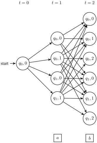
For any other step we calculate the value of ˆα recursively:
- Recursion Step:
if c -∆= 0 :
if c -∆> 0 :
ˆαt(q, c) =
Theorem 1. ˆαt(q, c) calculates Pr(o1:t, St|S0) correctly.
Second Phase: Normalized Forward
The second phase of the algorithm calculates αt(q, c): the joint probability distribution of the observation sequence o1:t and the hidden state-counter pair at step t being St = (q, c) under the condition that the initial configuration is S0 = (q0, 0) and the terminal configuration has to be ST = (qF , 0). Formally we write this as:
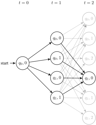
The way to compute this is to remove all paths from the trellis diagram from which ST = (qF , 0) cannot be reached in step T. Naturally, without normalization, the probabilities to take any of these paths is now Pr(ST |S0), and no longer 1, and we need to normalize the probabilities accordingly.
- Base Step:
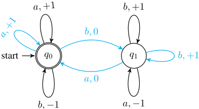
At the base step t = T , the calculation of normalization starts in the final state with zero counter ST = (qF , 0). The rest of the hidden state-counter pairs are discarded because our model only accepts a run that ends at such final configuration at t = T as shown in Figure 2. The accepting state is q1 with zero counter value in this example. The normalized probability of (q1, 0), according to the equation of the base step, is found by dividing the preliminary probability of the forward flow of (q1, 0) with the total probability of reaching the final configuration from the initial configuration.
There are three important points regarding the calculation of the normalized probability of valid paths. First is that the calculation starts from the final state with a zero counter value. Second is that the time step is decremented by one in each iteration. Therefore, in this phase, the normalization calculation at a particular time step t will be used when calculating the normalized probability as the time step t-1. The last point is that we need all the preliminary probability values of the forward flow that we calculated in the first phase.
Theorem 2. αt(q, c) computes correctly the joint probability P r(o1:t, St = (q, c)|S0, ST ).
3.2 Adaptation of Backward Algorithm
The adapted Backward algorithm computes the probability of the future observation ot+1:T conditioned on the value of St.
First Phase: Preliminary Backward Calculation
We calculate here, ˆ βt(q, c), the probability of reaching the terminal configuration at the final step T from a given configuration (q, c) at step t (given that we started at the initial configuration). Formally:
The computation starts at the designated final configuration ST = (qF , 0) at time t = T as shown in Figure 2 but the base and recursion steps are different from the normalization of adapted Forward calculation. For instance, we do not look at the emitted observations in this phase.
- Base Step:
- Recursion Step:
if c = 0 :
if c > 0 :
Theorem 3. ˆ βt(q, c) calculates Pr(ST |St = (q, c), S0) correctly.
Second Phase: Normalization Backward Flow
In this phase the probability of emitting the future observation sequence ot+1:T is calculated conditioned on the current configuration and that the terminal configuration is reached. Formally,βt(q, c) = P r(ot+1:T |St = (q, c), S0, ST )
The calculation of the normalization of the backward flow is started at the last time step T. The preliminary probability of the backward flow is needed here.
- Base Step:
- Recursion Step:
Theorem 4. βt(q, c) calculates correctly the probabilities P r(ot+1:T |St = (q, c), S0, ST ).
3.3 Adaptation of Baum-Welch Algorithm
It is worth to point out that the original Baum-Welch algorithm is a special case of the Expectation Maximization (EM) algorithm [Bilmes, 2000] therefore the same aspect is considered on the adapted version when the counter variable is taken into account. The adapted algorithm runs a procedure that finds a set of parameters that get closer and closer to the optimal model. It is repeating the following steps:
E-Step
In this step, there are two calculations where each takes into account the counter value.
Theorem 5. γt(q, c) = Pr(St|O, S0, ST ) is the calculation of the marginal posterior distribution of a hidden variable St = (q, c) where
Theorem 6. ξt((q′ , c′ ), (q, c)) = Pr(St-1, St|O, S0, ST ) calculates the joint posterior distribution of two successive hidden variables of the model where
and
M-Step
In the M-step, we use the posterior parameters (i.e., θ) to find new parameters (i.e., θ′ ) of the model that maximize the expected likelihood as estimated in the E-step. We can write the joint probability distribution over hidden, counter and observation variables as follows:
where
We consider multiple observation sequences to learn an optimal model. Here, D represents the number of observation sequences. We use Lagrange multipliers to obtain optimized
values for the model parameters. The updated formula for the emission matrix is
where I(o) denotes an indicator function which is 1 if ot = o is true, and 0 otherwise. The updated formulas for state transition matrices ˆ A0 and ˆ A+, respectively, are
4 Experiments
All algorithms here were implemented in Python and evaluated on Intel i7 3.3 GHz CPU with 16 GB RAM. We also implemented the standard algorithms (forward, backward, Baum-Welch) for HMMs ourselves for a fair comparison. The full source-code and the inputs used will be made freely available online.
We tested the algorithm on the following input. We first created 6 different models Hi = (Qi,Σi,A0i ,A+i ,Bi, q0, qF ), where i = 1, 2 . . . , 6. Model Hi has i + 1 states and Figure 2 shows Hi where the probability values are omitted. Each model has a structure similar to this example, which was picked in order to exhibit an interesting counting behavior from the model. The probabilities of transitions and observations A0i , A+i , and Bi were then randomly selected.
Then using each Hi, we created a random multi-set of observation sequences Oi(Hi, T, 20000) that contain 20000 observation sequences with a fixed length T = 16.
To simplify the comparison, we let the number of states of HMM to have 2.24 times more states (exactly √5 more) than the H1MM model that it is compared with. This is because to describe the transition matrix of H1MM with n states one needs 5n2 values, while HMM utilises only n2 values. This way we only compare models with the same total number of parameters and thus avoid the need to penalize the model with more parameters as one would do when using, e.g., Akaike or Bayesian information criteria for measuring the quality of models.
We noticed that both HMM and H1MM algorithm tend to get stuck in local minima very often. In order to avoid this, we followed the following procedure to train our models. We started with 100 different initial completely random (i.e., fully connected with probabilities picked uniformly at random) H1MMmodels (or HMMmodels). After each learning step, we discarded the bottom 25% of these models as measured by the value of their likelihood. Eventually we only had one model left that we trained until the learning process converged.
The running time of the learning process for HMMs Hi, i = 1, . . . , 6 took: 10 minutes, 30 minutes, 1 hour, 4
hours, 6 hours, 10 hours, respectively. The same task for the H1MM took: 1 hour, 6 hours, 22 hours, 79 hours, 218 hours, - (initialization was done by hand), respectively.
At the training step, the parameters of the model were reestimated using the adapted Baum-Welch algorithm discussed in the previous section. The learning algorithms has nested loops over the length T of the observation sequence, feasible maximum counter values M ≤ 12 T , and goes twice over the number of hidden states n = |Q| at each iteration step. Therefore, the complexity of the adapted Baum-Welch algorithm is O(n2TM), where the counter value cannot exceed the remaining length of the observation sequence; in particular M ≤ 1 2 T .
The learnt HMM and H1MM models were then compared with the original model. We chose as the performance metric the likelihood of a set of test observations, which were different from the observation sequences used in the learning process. We calculated the similarity score using the KullbackLeibler (KL) divergence.
Here, P(x) addresses the original likelihood distribution and Q(x) shows the likelihood distribution of the model to be analyzed for every variable x. This estimates the difference between two likelihood distributions. Only if two distributions match perfectly, the KL score is zero otherwise and the closer to 0 it is the better. As we can see in Table 1, our H1MM algorithms learnt almost perfectly the original model, while HMMs struggle to get any close. The price we pay for that is obviously the longer running time, but we are still much faster compared to using PCFGs instead. In fact, based on the running time of our learning algorithms for HMM and H1MM, we can extrapolate that, if we were to implement the standard cubic inside-outside learning algorithm for PCFGs, it would timeout already for H3.
| Model | H1 | H2 | H3 | H4 | H5 | H6 |
| H1MM | 0.008 | 0.0022 | 0.11 | 0.0027 | 0.0045 | 0.0064 |
| HMM | 4.94 | 5.44 | 5.24 | 5.26 | 6.799 | 5.11 |
Acknowledgements
- This project has received funding from the European Union's Horizon 2020 research and innovation programme under grant agreement No 956123. It has been supported by the EPSRC through the Programme Grant EP/V026887/1 (Digital navigation of chemical space for function).
@inproceedings{ijcai2022p673,
  title     = {Hidden 1-Counter Markov Models and How to Learn Them},
  author    = {Kurucan, Mehmet and Özbaltan, Mete and Schewe, Sven and Wojtczak, Dominik},
  booktitle = {Proceedings of the Thirty-First International Joint Conference on
               Artificial Intelligence, {IJCAI-22}},
  publisher = {International Joint Conferences on Artificial Intelligence Organization},
  editor    = {Luc De Raedt},
  pages     = {4857--4863},
  year      = {2022},
  month     = {7},
  note      = {Main Track},
  doi       = {10.24963/ijcai.2022/673},
  url       = {https://doi.org/10.24963/ijcai.2022/673},
}
TY - CPAPER TI - Hidden 1-Counter Markov Models and How to Learn Them AU - Kurucan, Mehmet AU - Özbaltan, Mete AU - Schewe, Sven AU - Wojtczak, Dominik T2 - Proceedings of the Thirty-First International Joint Conference on Artificial Intelligence, IJCAI-22 PB - International Joint Conferences on Artificial Intelligence Organization PY - 2022 SP - 4857 EP - 4863 DO - 10.24963/ijcai.2022/673 UR - https://doi.org/10.24963/ijcai.2022/673 ER -Copied
Machine-readable versions of this paper, for tools and AI agents:





