
Depth-Relative Self Attention for Monocular Depth Estimation
Proceedings of the Thirty-Second International Joint Conference on Artificial Intelligence. Main Track. Pages 1396-1404.
https://doi.org/10.24963/ijcai.2023/155
Keywords
- Computer Vision: CV: Applications
- Computer Vision: CV: Machine learning for vision
Abstract
Monocular depth estimation is very challenging because clues to the exact depth are incomplete in a single RGB image. To overcome the limitation, deep neural networks rely on various visual hints such as size, shade, and texture extracted from RGB information. However, we observe that if such hints are overly exploited, the network can be biased on RGB information without considering the comprehensive view. We propose a novel depth estimation model named RElative Depth Transformer (RED-T) that uses relative depth as guidance in self-attention. Specifically, the model assigns high attention weights to pixels of close depth and low attention weights to pixels of distant depth. As a result, the features of similar depth can become more likely to each other and thus less prone to misused visual hints. We show that the proposed model achieves competitive results in monocular depth estimation benchmarks and is less biased to RGB information. In addition, we propose a novel monocular depth estimation benchmark that limits the observable depth range during training in order to evaluate the robustness of the model for unseen depths.
- [Agarwal and Arora, 2023] Ashutosh Agarwal and Chetan Arora. Attention attention everywhere: Monocular depth prediction with skip attention. In Proceedings of the IEEE/CVF Winter Conference on Applications of Computer Vision, pages 5861-5870, 2023.
- [Atapour-Abarghouei and Breckon, 2018] Amir Atapour- Abarghouei and Toby P Breckon. Real-time monocular depth estimation using synthetic data with domain adaptation via image style transfer. In Proceedings of the IEEE conference on computer vision and pattern recognition, pages 2800-2810, 2018.
- [Bhat et al., 2021] Shariq Farooq Bhat, Ibraheem Alhashim, and Peter Wonka. Adabins: Depth estimation using adap- tive bins. In Proceedings of the IEEE/CVF Conference on Computer Vision and Pattern Recognition, pages 4009- 4018, 2021.
- [Chen et al., 2020] Zuyao Chen, Qianqian Xu, Runmin Cong, and Qingming Huang. Global context-aware progressive aggregation network for salient object detection. In Pro- ceedings of the AAAI conference on artificial intelligence, volume 34, pages 10599-10606, 2020.
- [Deng et al., 2009] Jia Deng, Wei Dong, Richard Socher, Li- Jia Li, Kai Li, and Li Fei-Fei. Imagenet: A large-scale hierarchical image database. In 2009 IEEE conference on computer vision and pattern recognition, pages 248-255.
- [Eigen et al., 2014] David Eigen, Christian Puhrsch, and Rob Fergus. Depth map prediction from a single image using a multi-scale deep network. Advances in neural information processing systems, 27, 2014.
- [Fu et al., 2018] Huan Fu, Mingming Gong, Chaohui Wang, Kayhan Batmanghelich, and Dacheng Tao. Deep ordinal regression network for monocular depth estimation. In Proceedings of the IEEE conference on computer vision and pattern recognition, pages 2002-2011, 2018.
- [Geiger et al., 2011] Andreas Geiger, Julius Ziegler, and Christoph Stiller. Stereoscan: Dense 3d reconstruction in real-time. In 2011 IEEE intelligent vehicles symposium (IV), pages 963-968. Ieee, 2011.
- [Geiger et al., 2012] Andreas Geiger, Philip Lenz, and Raquel Urtasun. Are we ready for autonomous driving? the kitti vision benchmark suite. In 2012 IEEE conference on computer vision and pattern recognition, pages 3354-3361. IEEE, 2012.
- [Geiger et al., 2013] Andreas Geiger, Philip Lenz, Christoph Stiller, and Raquel Urtasun. Vision meets robotics: The kitti dataset. The International Journal of Robotics Research, 32(11):1231-1237, 2013.
- [Girshick et al., 2014] Ross Girshick, Jeff Donahue, Trevor Darrell, and Jitendra Malik. Rich feature hierarchies for accurate object detection and semantic segmentation. In Proceedings of the IEEE conference on computer vision and pattern recognition, pages 580-587, 2014.
- [Huynh et al., 2020] Lam Huynh, Phong Nguyen-Ha, Jiri Matas, Esa Rahtu, and Janne Heikkilä. Guiding monoc- ular depth estimation using depth-attention volume. In European Conference on Computer Vision, pages 581-597. Springer, 2020.
- [Izadi et al., 2011] Shahram Izadi, David Kim, Otmar Hilliges, David Molyneaux, Richard Newcombe, Push- meet Kohli, Jamie Shotton, Steve Hodges, Dustin Freeman, Andrew Davison, et al. Kinectfusion: real-time 3d recon- struction and interaction using a moving depth camera. In Proceedings of the 24th annual ACM symposium on User interface software and technology, pages 559-568, 2011.
- [Kim et al., 2002] Kwang In Kim, Keechul Jung, and Jin Hyung Kim. Color texture-based object detection: an application to license plate localization. In International Workshop on Support Vector Machines, pages 293-309. Springer, 2002.
- [Kingma and Ba, 2014] Diederik P Kingma and Jimmy Ba. Adam: A method for stochastic optimization. arXiv preprint arXiv:1412.6980, 2014.
- [Kolesnikov et al., 2020] Alexander Kolesnikov, Lucas Beyer, Xiaohua Zhai, Joan Puigcerver, Jessica Yung, Sylvain Gelly, and Neil Houlsby. Big transfer (bit): General visual representation learning. In European conference on computer vision, pages 491-507. Springer, 2020.
- [Kramer and MacKinnon, 1993] Bernhard Kramer and An- gus MacKinnon. Localization: theory and experiment. Reports on Progress in Physics, 56(12):1469, 1993.
- [Lee and Kim, 2019] Jae-Han Lee and Chang-Su Kim. Monocular depth estimation using relative depth maps. In Proceedings of the IEEE/CVF Conference on Computer Vision and Pattern Recognition, pages 9729-9738, 2019.
- [Lee et al., 2019] Jin Han Lee, Myung-Kyu Han, Dong Wook Ko, and Il Hong Suh. From big to small: Multi-scale local planar guidance for monocular depth estimation. arXiv preprint arXiv:1907.10326, 2019.
- [Li et al., 2022a] Zhenyu Li, Zehui Chen, Xianming Liu, and Junjun Jiang. Depthformer: Exploiting long-range corre- lation and local information for accurate monocular depth estimation. arXiv preprint arXiv:2203.14211, 2022.
- [Li et al., 2022b] Zhenyu Li, Xuyang Wang, Xianming Liu, and Junjun Jiang. Binsformer: Revisiting adaptive bins for monocular depth estimation. arXiv preprint arXiv:2204.00987, 2022.
- [Liang et al., 2021] Jingyun Liang, Jiezhang Cao, Guolei Sun, Kai Zhang, Luc Van Gool, and Radu Timofte. Swinir: Image restoration using swin transformer. In Proceedings of the IEEE/CVF International Conference on Computer Vision, pages 1833-1844, 2021.
- [Lin et al., 2017] Tsung-Yi Lin, Piotr Dollár, Ross Girshick, Kaiming He, Bharath Hariharan, and Serge Belongie. Fea- ture pyramid networks for object detection. In Proceedings of the IEEE conference on computer vision and pattern recognition, pages 2117-2125, 2017.
- [Liu et al., 2021] Ze Liu, Yutong Lin, Yue Cao, Han Hu, Yix- uan Wei, Zheng Zhang, Stephen Lin, and Baining Guo. Swin transformer: Hierarchical vision transformer using shifted windows. In Proceedings of the IEEE/CVF Inter- national Conference on Computer Vision, pages 10012- 10022, 2021.
- [Ming et al., 2021] Yue Ming, Xuyang Meng, Chunxiao Fan, and Hui Yu. Deep learning for monocular depth estimation: A review. Neurocomputing, 438:14-33, 2021.
- [Ranftl et al., 2021] René Ranftl, Alexey Bochkovskiy, and Vladlen Koltun. Vision transformers for dense prediction. In Proceedings of the IEEE/CVF International Conference on Computer Vision, pages 12179-12188, 2021.
- [Redmon and Farhadi, 2018] Joseph Redmon and Ali Farhadi. Yolov3: An incremental improvement. arXiv preprint arXiv:1804.02767, 2018.
- [Saxena et al., 2007] Ashutosh Saxena, Jamie Schulte, An- drew Y Ng, et al. Depth estimation using monocular and stereo cues. In IJCAI, volume 7, pages 2197-2203, 2007. IJCAI
- [Silberman et al., 2012] Nathan Silberman, Derek Hoiem, Pushmeet Kohli, and Rob Fergus. Indoor segmentation and support inference from rgbd images. In European conference on computer vision, pages 746-760. Springer, 2012.
- [Tan et al., 2020] Mingxing Tan, Ruoming Pang, and Quoc V Le. Efficientdet: Scalable and efficient object detection. In Proceedings of the IEEE/CVF conference on computer vision and pattern recognition, pages 10781-10790, 2020.
- [Tompson et al., 2015] Jonathan Tompson, Ross Goroshin, Arjun Jain, Yann LeCun, and Christoph Bregler. Efficient object localization using convolutional networks. In Pro- ceedings of the IEEE conference on computer vision and pattern recognition, pages 648-656, 2015.
- [Vazquez et al., 2010] Eduard Vazquez, Ramon Baldrich, Joost Van de Weijer, and Maria Vanrell. Describing re- flectances for color segmentation robust to shadows, high- lights, and textures. IEEE Transactions on Pattern Analysis and Machine Intelligence, 33(5):917-930, 2010.
- [Wang et al., 2019] Yan Wang, Wei-Lun Chao, Divyansh Garg, Bharath Hariharan, Mark Campbell, and Kilian Q Weinberger. Pseudo-lidar from visual depth estimation: Bridging the gap in 3d object detection for autonomous driving. In Proceedings of the IEEE/CVF Conference on Computer Vision and Pattern Recognition, pages 8445- 8453, 2019.
- [Wofk et al., 2019] Diana Wofk, Fangchang Ma, Tien-Ju Yang, Sertac Karaman, and Vivienne Sze. Fastdepth: Fast monocular depth estimation on embedded systems. In 2019 International Conference on Robotics and Automa- tion (ICRA), pages 6101-6108. IEEE, 2019.
- [You et al., 2019] Yurong You, Yan Wang, Wei-Lun Chao, Divyansh Garg, Geoff Pleiss, Bharath Hariharan, Mark Campbell, and Kilian Q Weinberger. Pseudo-lidar++: Ac- curate depth for 3d object detection in autonomous driving. arXiv preprint arXiv:1906.06310, 2019.
- [Yu et al., 2020] Changqian Yu, Jingbo Wang, Changxin Gao, Gang Yu, Chunhua Shen, and Nong Sang. Context prior for scene segmentation. In Proceedings of the IEEE/CVF Conference on Computer Vision and Pattern Recognition, pages 12416-12425, 2020.
- [Yuan et al., 2022] Weihao Yuan, Xiaodong Gu, Zuozhuo Dai, Siyu Zhu, and Ping Tan. New crfs: Neural window fully-connected crfs for monocular depth estimation. arXiv preprint arXiv:2203.01502, 2022.
- [Yucel et al., 2021] Mehmet Kerim Yucel, Valia Dimaridou, Anastasios Drosou, and Albert Saa-Garriga. Real-time monocular depth estimation with sparse supervision on mobile. In Proceedings of the IEEE/CVF Conference on Computer Vision and Pattern Recognition, pages 2428- 2437, 2021.
- [Zhao et al., 2021] Jiawei Zhao, Ke Yan, Yifan Zhao, Xi- aowei Guo, Feiyue Huang, and Jia Li. Transformer-based dual relation graph for multi-label image recognition. In Proceedings of the IEEE/CVF International Conference on Computer Vision, pages 163-172, 2021.
- [Zhong and Jain, 2000] Yu Zhong and Anil K Jain. Object localization using color, texture and shape. Pattern Recog- nition, 33(4):671-684, 2000.
References were extracted automatically from the PDF and may contain errors.
Full text extracted automatically from the PDF; figures, tables and equations may differ. The PDF is the version of record.
1 Introduction
Depth estimation, a task to estimate the distance from the viewpoint, is one of the most important tasks in computer vision having a variety of applications such as autonomous driving [Wang et al., 2019; You et al., 2019], object localization [Kramer and MacKinnon, 1993; Tompson et al., 2015], 3D reconstruction [Geiger et al., 2011; Izadi et al., 2011], to name just a few. Due to the cost and power consumption of depth measuring sensors (e.g., LiDAR, Time-of-Flight), a single RGB image has been used for this task in many realworld applications [Atapour-Abarghouei and Breckon, 2018; Yucel et al., 2021; Wofk et al., 2019]. The major difficulty of this task, monocular depth estimation (MDE), is that the task is ill-posed since there are multiple answers for the given scene. Recently, deep neural networks alleviated this problem by exploiting diverse visual clues such as relative size, brightness, patterns, and vanishing point extracted from an RGB image. It has been shown that these visual clues, collectively called
"visual hints", are useful in predicting the depth [Saxena et al., 2007; Ming et al., 2021].
In order to improve the quality of visual hints, a pre-trained network referred to as 'backbone' has been widely used. Recently, depth estimation performance has been substantially improved [Li et al., 2022a; Yuan et al., 2022] due to the diverse and complex RGB-based visual features obtained from the large-scale backbone networks [Girshick et al., 2014; Kolesnikov et al., 2020; Liu et al., 2021]. However, we observe that some visual information such as painted surfaces, a patterned carpet, and reflected sunlight sometimes provide false signals to the network and degrade the accuracy of the predicted depth (see Figure 1). While the visual hints are useful to some extent, they would do more harm than good when models become overly dependent on such information. In the sequel, we call the visual hints that confuse the model and therefore have an adverse effect on the depth estimation as "visual pits". For example, in Figure 1(a), the dark paint of the truck affects the model such that the truck appears farther away than it really is. Clearly, visual pits can be a potential risk factor for the autonomous driving system.
To reduce the negative effect of visual pits, we should design the system such that the extracted features are more related to depth while less dependent on RGB-based information. In other words, we expect that the features corresponding to pixels of similar depths to be similar. As an enabler to achieve this goal, we exploit the relative depth, a difference between the depth of two pixels. If the relative depth between two pixels is small, the model should generate similar features regardless of their RGB attributes and spatial distances in 2D image 1 . When this property is satisfied, even though the two complementary information (i.e., RGB and depth) make contradictory predictions, we can use the relative depth as guidance in estimating the correct depth. For example, in Figure 1(b), the model is confused by the reflected sunlight, resulting in an incorrect prediction that the upper part of the pillar is farther than its real depth. Even in this case, using the relative depth between the lower and upper parts of the pillar is small, the model can figure out that both parts are actually at the same depth.
1 In order to make a clear distinction between the distance in the 2D image and the real world, we exclusively use the terms 'near/far' for the former, and 'close/distant' for the latter.
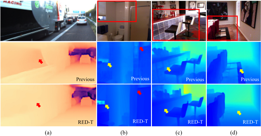
In this paper, we propose a novel MDE model referred to as RElative Depth Transformer (RED-T). The key idea of RED-T is to exploit the relative depth as guidance in computing the self-attention weights. To this end, we design the depth-relative attention module on top of the backbone. Using the relative depth information, this module modifies the self-attention weight in two steps. First, we gather the relative depth information to determine which pixels should be similar in the feature domain. Second, we adjust the self-attention weight based on the relative depth; large (small) attention weights for pixels of small (large) relative depths. We expect that features with large attention weights are more or less similar to each other since the self-attention mechanism is basically a weighted sum of features. In fact, through the proposed depth-aware self-attention process, the features corresponding to pixels with small relative depths will be close to each other in the feature domain, even if their RGB values are different. Whereas, if the relative depth is large, the features would be distinct although their corresponding RGB attributes may look alike.
To demonstrate the negative effect of visual pits, we propose a new practical MDE environment termed range-restricted MDE. In the conventional depth estimation benchmarks, the target depth range is the same for both training and evaluation. To make things worse, the annotated depth data has limitations in range (e.g., 10m for NYU-v2 [Silberman et al., 2012] and 80m for KITTI [Geiger et al., 2013] datasets). However, in real-world scenarios, we should estimate the depth of distant objects correctly even if their depths are not specified in the training data. When the model only learns the correlation between RGB attributes and limited depths, the model would inaccurately estimate the unseen depths to seen depths highly dependent on the RGB information, which will intensify the adverse influence of visual pits on such unseen depth range. In the proposed environments, we erase the depth labels of a certain range as if they are not annotated in training data. For example, for the data with a depth range of 0 ∼ 80m, we remove the training labels in 40 ∼ 80m and evaluate the model with the full range (0 ∼ 80m). In our evaluations, we show that RED-T predicts not only the learned depth but also the outof-range depth more accurately than previous state-of-the-art MDE models.
The contributions of this work are as follows:
- We employ relative depth, a difference between the depth of pixels, as guidance to solve the problem of visual pit. To the best of our knowledge, we are the first to tackle the negative effect of visual information in MDE.
- We propose a novel depth-relative attention that adjusts the self-attention weight based on the relative depth. In essence, the proposed mechanism guides feature such that the depth is more considered than RGB information.
- Using two MDE datasets (KITTI & NYU-v2), we evaluate RED-T and show that the proposed RED-T outperforms the recent MDE models that use the same backbone in all metrics for the extremely competitive KITTI dataset.
- To evaluate the performance of MDE models in practical environments, we suggest new depth estimation scenarios that restrict observable depth range during training. We show that the depth-relative attention bias makes the model more robust in estimating unseen depth ranges.
2 RelatedWork
Adversarial Effect of Visual Pits. Visual information extracted from an RGB image such as color, texture, style, and brightness is known to be helpful in object detection, semantic segmentation, and super resolution [Kim et al., 2002; Liang et al., 2021; Zhong and Jain, 2000], etc. However, this perceptual information is not always reliable, especially when the goal of the task is to generate output in a non-RGB domain with RGB input. For example, in the image segmentation task, the pixels corresponding to the same class must produce the same mask even if their RGB values are different. Previous work pointed out that the physical effects of illumination, shadow, shading, and highlights can cause considerable noise in the image segmentation output [Vazquez et al., 2010]. Likewise, in MDE, visual pits such as patterned surfaces, dark screens, and reflections in the mirror can disturb the depth estimation process. To avoid the failures caused by visual pits, we exploit the relative depth information such that the MDE model can focus more on depth-related information.
Relative Depth. Several studies have used relative depth information for depth estimation [Huynh et al., 2020; Lee and Kim, 2019], but their works are very distinct from ours. The main difference to the referred papers is that 1) we investigated the 'visual pit' problem which has not been studied before and 2) we exploited the novel depth-relative attention bias instead of the position-relative bias. We note that studies [Huynh et al., 2020; Lee and Kim, 2019] that introduced relative depth in the feature extraction are difficult to apply when dense depth labels are not given. For example, the former does not show the performance on KITTI, a dataset where only a few pixels are labeled sparsely. Also, the latter mentioned that the training process was less reliable on KITTI as their labels are not annotated. In contrast, as can be observed in restricted label experiments, our method works well on much sparser scenarios than the original KITTI. Please also note that we are the first to exploit relative depth information among the models that use the same Swin backbone [Li et al., 2022a; Li et al., 2022b; Agarwal and Arora, 2023].
3 RED-T: RElative Depth Transformer
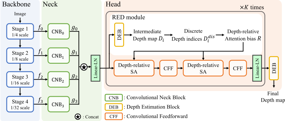
In this section, we discuss three components, backbone, neck, and head, of the proposed RED-T. Figure 2 illustrates the overall architecture of the model.
3.1 Monocular Depth Estimation
Let H and W be the height and width of the image, then the MDE model takes a single RGB image I ∈ RH×W×3 as input and returns the estimated depth map D ∈ RH×W×1 . Each element of D represents a distance d from the viewpoint. Because the ground truth depth map D∗ contains only a few annotated pixels, the loss is computed on those pixels in the training stage.
3.2 Backbone: Position-relative Transformer
As a backbone, we use Swin Transformer (Swin) [Liu et al., 2021], a multi-stage Transformer whose self-attention (SA) is computed with non-overlapping local windows. In Swin, SA between n pixels is calculated as:
where h is the attention head index over the total number of heads Nh and dh is the attention head dimension. Qh,Kh, Vh ∈ Rn×dh are the query, key, value matrices for the h-th attention head, respectively, and Ah ∈ Rn×n is the attention weight. To promote the spatial relationship between pixels, Swin adds the relative positional attention bias Bh ∈ Rn×n to the attention weight. Note that Bh is unrelated to the content and depends only on the difference in coordinates (i.e., spatial location) between pixels.
3.3 Neck: Parallel Multi-scale Aggregation
The neck performs parallel processing of the multi-scale backbone features with different scales and then stacks them together at the highest resolution (largest scale). To ensure that the scale of features is the same, features are upsampled to the highest resolution. Let f{0,1,2,3} be the image features extracted from the backbone corresponding to 1/4, 1/8, 1/16, 1/32 scales, then each image feature fi is passed through a convolutional block. The block takes i-th feature fi as an input and then returns the processed feature gi. The generated features g{0,1,2,3} are concatenated and passed through an additional linear layer followed by layer normalization.
Traditional feature pyramid network (FPN) merges multiscale features one after another, from the smallest scale features to the largest scale ones [Lin et al., 2017; Tan et al., 2020; Redmon and Farhadi, 2018]. Since FPN merges the multiscale features sequentially, global information from smallscale features can be blurred during the hierarchical process [Chen et al., 2020; Yu et al., 2020]. This might cause a loss of the global information presumably obtained from low-resolution features in local pixels. Our neck architecture overcomes the potential weakness by combining all scales simultaneously.
3.4 Head: Depth-relative Transformer
The relative depth r between two pixels x1 and x2 is the difference between their depth values d1 and d2, that is r(x1, x2) = d1 - d2. To obtain the relative depth between every pair of pixels, each pixel should have its own depth value; however, such a dense depth map is not available during the training and even the GT map does not contain depth values for all pixels. To deal with the issue, we generate the intermediate dense depth map prediction and use it to compute the relative depth information. The relative depth information is then used to predict the enhanced depth map. This process can be interpreted as self-guided bootstrapping; RED-T repeats this cycle multiple times (K times) to improve the intermediate depth maps progressively.
The detailed process of each cycle is as follows:
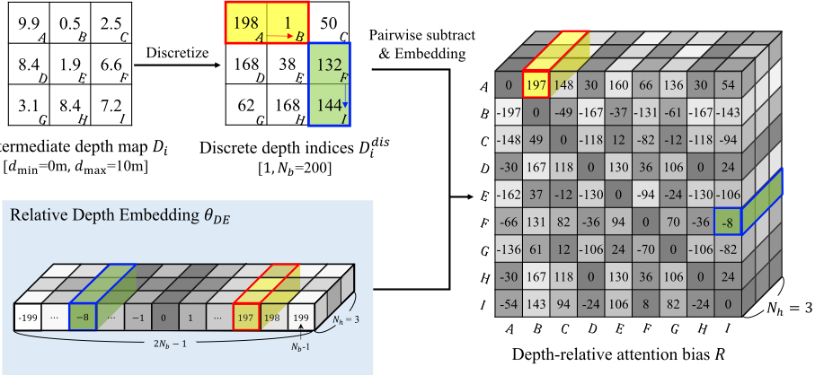
Discretization. In the i-th iteration, the model produces an intermediate depth map Di. Since Di is a real-valued dense depth map, every pixel of Di has its own estimated depth value and thus every relative depth can be computed. Then, we discretize depth values by uniformly splitting the min-max depth range, where the number of bins Nb is a hyperparameter. This discretization converts depth map Di into Ddis i , as illustrated in Figure 3. Note that the number of possible relative depths after the discretization is 2Nb - 1, from -Nb + 1 to Nb -1. If we increase Nb in the discretization process, a more fine-grained granularity of relative depth can be obtained. We empirically observed that 128 bins are sufficient.
Parameterization. We parameterize the possible relative depths as embedding parameters θDE ∈ R(2Nb-1)×Nh (see Figure 3). The goal of this parameterization is to map a raw relative depth to a trainable parameter that can be simultaneously trained with other parameters. By doing so, the effect of relative depth on the attention weight can be automatically adopted for performance during training. Note that the parameter size of θDE is quite small (about 2K per each self-attention module) although different attention head uses different embedding parameters.
Pairwise subtraction &Embedding. For every pixel pair, we perform a pairwise subtraction of two discretized depth values fromDdis i and then take the corresponding embedding parameter from θDE to construct the depth-relative attention bias R. For example, in Figure 3, the pairwise subtraction outputs 197 by subtracting 198(A) and 1(B), which are discretized depths. Then, the vector corresponding to the index 197 is taken from θDE to (A, B) point of R. The R represents the relationship between pixels in terms of their depth difference, or relative depth. Note that each entry of R only depends on the relative depth between pixels and not on their visual features.
Depth-relative Self-attention. Instead of using the conventional relative positional attention bias B (see Eq. (1)), we incorporate the relative depth attention bias R as below:
This novel depth-relative SA mechanism encourages pixels of similar depth to focus more on each other. By assigning higher attention weight to features of similar depth (small relative depth), the features can be more correlated to depth. Thus, the model can less affected by visual pits such as patterns or colors.
3.5 Other Details
Relative Depth Computation. From earlier trials, we find that the uniform separation of depth range works well and performs better than the log-uniform partitioning as suggested in DORN [Fu et al., 2018]. Different depth-relative SA blocks equip their own relative depth embedding parameters θDE so that each SA can learn diverse depth relationships.
Training loss. The total loss Ltotal is the scale-invariant loss [Eigen et al., 2014] averaged over all intermediate depth maps Di∈{0,1,...K-1} and the final depth map DK.
where hi,x = log d∗x - log di,x and T is the number of valid GT labels. The loss for each depth map is calculated by the same equation above, reducing the possibility of the wrong prediction being amplified through iterations. We set λ=0.85 and α=10 following previous works [Bhat et al., 2021; Yuan et al., 2022].
4 Experiment
4.1 Dataset
NYU-v2 [Silberman et al., 2012] dataset includes pairs of RGB images and depth maps on 464 indoor scenes, which are separated into 120K training samples from 249 scenes and 654 testing samples from 215 scenes. The range of depth labels is up to 10 meters. We train our model on 50K subset following previous work [Yuan et al., 2022].
KITTI [Geiger et al., 2013] dataset consists of paired RGB images and corresponding depth maps obtained by a 3D laser scanner on 61 outdoor scenes while driving. The range of depth annotations is up to 80 meters. We apply two mainly used training/testing dataset splits. First, following the Eigen split setting [Eigen et al., 2014], we train our model with about 26K samples from 32 scenes and test on 687 samples from 29 scenes. Second, for the online depth prediction configuration [Geiger et al., 2012], we use 72K training samples, 6K validation samples, and 500 testing samples.
4.2 Implementation Details
We employ Swin-Large as a backbone, pre-trained on ImageNet-22K dataset [Deng et al., 2009] with an input image size of 224 and window size of 7. Each stage of the convolutional neck produces 512-channel feature maps, which are then concatenated and projected to 512 channels. The number of depth-relative SA heads is set to 8 and their window size and shift size is set to 8 and 4, respectively. We set K = 3 and Nb = 128 as default. The size of the output depth map is the 1/4 scale of the input image, which is then resized to the full resolution.
We use AdamW optimizer [Kingma and Ba, 2014] with a learning rate of 1e-4, (β1, β2) of (0.9, 0.999), and a weight decay of 0.1. The learning rate starts at 4e-6, increases to the maximum value for 25% of the total iterations, and then decreases to 1e-6. We train our model with a batch size of 16 for 24 epochs on 8× NVIDIA A5000 24GB GPUs. The gradient is accumulated every 2 batches and clipped to the maximum gradient norm of 0.1. Please see the Appendix for details about data pre-processing, augmentation, metrics, and evaluation procedure.
4.3 Depth Estimation Performance
Table 1 shows the MDE performance on the NYU-v2 dataset. Despite the fact that several models employ the same or larger backbones than RED-T or exploit additional data during training [Ranftl et al., 2021], RED-T achieves higher or comparable results in most of the metrics. In particular, RED-T reduces 'Abs Rel' and 'log 10' errors by 4.2% and 4.9% compared to NeWCRFs [Yuan et al., 2022], respectively.
Table 2 presents the performance on KITTI Eigen split dataset. RED-T outperforms previous works in every metric; especially, RED-T achieves lower relative errors ('Abs Rel' and 'Sq Rel') and absolute errors ('RMSE' and 'RMSE log'). We also evaluate RED-T on the KITTI official split which measures the performance on the official server. As shown in Table 3, RED-T surpasses competitors by a large margin, especially in 'Abs Rel' and 'iRMSE' metrics.
The number of parameters of models that use the same SwinL backbone is 270.4M, 273.8M, and 248.3M for NewCRFs, DepthFormer, and RED-T, respectively. Note that the backbone contains 195.0M parameters.
4.4 Qualitative Evaluation
In Figure 1(a), a truck is painted with diverse colors (i.e, black, gray, white) on its surface. Although the depth of the surface continuously changes, in previous work [Bhat et al., 2021], undesired change in depth appears in the estimated output due to the color difference. Another example is a kitchen counter wall decorated with a square pattern (Figure 1(c)). While the depth of the wall should change smoothly, in the previous work, the pattern erroneously stands out in the depth map. Thanks to the relative depth that help distinguish visual pits from visual hints, RED-T is robust to such obstacles. In other words, RED-T can accurately predict the depth of an object while much less affected by its visual appearance in 2D images. Please check the Appendix for more qualitative comparisons.
| Method | Backbone | Abs Rel↓ | RMSE↓ | log 10 ↓ | δ1 ↑ | δ2 ↑ | δ3 ↑ |
|---|---|---|---|---|---|---|---|
| DORN [Fu et al., 2018] | ResNet-101 | 0.115 | 0.509 | 0.051 | 0.828 | 0.965 | 0.992 |
| BTS [Lee et al., 2019] | DenseNet-161 | 0.110 | 0.392 | 0.047 | 0.885 | 0.978 | 0.994 |
| TransDepth [Zhao et al., 2021] | R-50+ViT-B† | 0.106 | 0.365 | 0.045 | 0.900 | 0.983 | 0.996 |
| DPT [Ranftl et al., 2021] | R-50+ViT-B‡ | 0.110 | 0.357 | 0.045 | 0.904 | 0.988 | 0.998 |
| Adabins [Bhat et al., 2021] | E-B5+mini-ViT | 0.103 | 0.364 | 0.044 | 0.903 | 0.984 | 0.997 |
| NeWCRFs [Yuan et al., 2022] | Swin-L† | 0.095 | 0.334 | 0.041 | 0.922 | 0.992 | 0.998 |
| DepthFormer [Li et al., 2022a] | R-50-C1+Swin-L† | 0.096 | 0.339 | 0.041 | 0.921 | 0.989 | 0.998 |
| BinsFormer∗ [Li et al., 2022b] | Swin-L† | 0.094 | 0.330 | 0.040 | 0.925 | 0.989 | 0.997 |
| RED-T (Ours) | Swin-L† | 0.091 | 0.328 | 0.039 | 0.926 | 0.990 | 0.998 |
| Method | Abs Rel↓ | Sq Rel↓ | RMSE↓ | RMSE log↓ | δ1 ↑ | δ2 ↑ | δ3 ↑ |
|---|---|---|---|---|---|---|---|
| DORN [Fu et al., 2018] | 0.072 | 0.307 | 2.727 | 0.120 | 0.932 | 0.984 | 0.994 |
| BTS [Lee et al., 2019] | 0.059 | 0.245 | 2.756 | 0.096 | 0.956 | 0.993 | 0.998 |
| TransDepth [Zhao et al., 2021] | 0.064 | 0.252 | 2.755 | 0.098 | 0.956 | 0.994 | 0.999 |
| DPT [Ranftl et al., 2021] | 0.062 | - | 2.573 | 0.092 | 0.959 | 0.995 | 0.999 |
| Adabins [Bhat et al., 2021] | 0.058 | 0.190 | 2.360 | 0.088 | 0.964 | 0.995 | 0.999 |
| NeWCRFs [Yuan et al., 2022] | 0.052 | 0.155 | 2.129 | 0.079 | 0.974 | 0.997 | 0.999 |
| DepthFormer [Li et al., 2022a] | 0.052 | 0.158 | 2.143 | 0.079 | 0.975 | 0.997 | 0.999 |
| BinsFormer [Li et al., 2022b] | 0.052 | 0.151 | 2.098 | 0.079 | 0.974 | 0.997 | 0.999 |
| RED-T (Ours) | 0.050 | 0.146 | 2.080 | 0.077 | 0.976 | 0.997 | 0.999 |
| Method | SILog ↓ | Abs Rel↓ | Sq Rel ↓ | iRMSE ↓ |
|---|---|---|---|---|
| DORN | 11.77 | 8.78 | 2.23 | 12.98 |
| BTS | 11.67 | 9.04 | 2.21 | 12.23 |
| BANet | 11.55 | 9.34 | 2.31 | 12.17 |
| PWA | 11.45 | 9.05 | 2.30 | 12.32 |
| NeWCRFs | 10.39 | 8.37 | 1.83 | 11.03 |
| DepthFormer | 10.46 | 8.54 | 1.82 | 11.17 |
| RED-T (Ours) | 10.36 | 8.11 | 1.92 | 10.82 |
5 Range-restrictedMDE
5.1 Motivation
As mentioned in Section 1, the harm of visual pits would be amplified when the model only exploits RGB information for depth estimation. Unfortunately, this is an inherent problem for MDE because 1) the model only takes a single RGB image as input, and 2) the range of the annotated depth label is limited. Therefore, for certain depth ranges that the model did not observe during training, the model solely depends on RGB values including visual pits which hurts the performance.
5.2 Task Specification
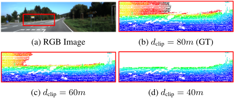
We propose a new MDE task that only a limited range of GT labels is given during training. Specifically, let the GT labels in test data d∗ ∈ [dmin, dmax], then we remove labels larger than dclip and use only [dmin, dclip] during training phase. As a result, the model should predict both seen and unseen depth ranges during the test phase. Figure 4 shows examples of the restricted GT maps corresponding to different dclip values.
| Metric | Model | ∼40m | ∼60m | ∼80m |
|---|---|---|---|---|
| Abs Rel↓ | AdaBins NeWCRFs RED-T | 0.091 0.058 0.055 | 0.077 0.054 0.050 | 0.058 0.052 0.050 |
| RMSE↓ | AdaBins NeWCRFs RED-T | 4.048 3.616 3.212 | 2.697 2.336 2.232 | 2.375 2.129 2.080 |
| δ1 ↑ | AdaBins NeWCRFs RED-T | 0.935 0.955 0.957 | 0.956 0.970 0.974 | 0.964 0.974 0.976 |
| Metric | Rel.bias | ∼2m | ∼4m | ∼6m | ∼8m |
|---|---|---|---|---|---|
| Abs Rel↓ | ✗ ✓ | 0.365 0.307 | 0.109 0.106 | 0.094 0.092 | 0.091 0.091 |
| RMSE↓ | ✗ ✓ | 1.882 1.537 | 0.533 0.504 | 0.366 0.360 | 0.337 0.331 |
| δ1 ↑ | ✗ ✓ | 0.471 0.491 | 0.868 0.878 | 0.917 0.919 | 0.925 0.925 |
5.3 Experimental Results
We conduct experiments on the KITTI dataset, where dmax = 80m, with two configurations of dclip ∈ {40m, 60m}. Table 4 shows that RED-T achieves much lower performance degradation than previous models. In dclip = 60m setting, RED-T achieves zero performance loss in the 'Abs Rel' metric and 7.3% reduction in 'RMSE' metric, while AdaBins suffers from 32.8% and 13.6% performance loss, respectively. We claim that RED-T is robust to unseen depth range because the model can avoid visual pits by actively incorporating the relative depth information in the model design.
5.4 Effectiveness of Relative Bias
To highlight the importance of the relative depth, we repeat the same experiments without relative bias (i.e., forcing R = 0) on the NYU dataset. In Table 5, RED-T without depth-relative attention guidance shows 1) worse performance and 2) larger relative performance decay compared to the proposed RED-T. The gap between the RED-T with and without relative bias becomes larger as the observable depth range (dclip) decreases.
In addition, we measure the RMSE as a function of distance in various scenarios. In Figure 5(a), models trained by a restricted depth range show much larger error compared to the baseline (i.e., the model trained on full depth range) in unseen (depth) ranges. We observe that relative bias improves the generalization capability of the model in unseen ranges. Furthermore, in Figure 5(b), we show that multiple iterations of depth-relative processing in the head consistently reduce the error. Specifically, the RMSE is reduced by 2.1%, 4.6%, and 10.5% as the number of iterations k increases.
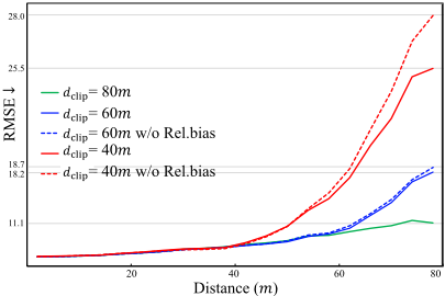
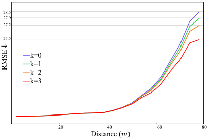
Figure 5: Fine-grained depth estimation results of range-restricted MDE experiments on the KITTI dataset.
One may think that the improvement of the relative bias is not dramatic on conventional depth estimation metrics. We argue that current metrics do not sufficiently express the negative effect of visual pits. First, the metric values are averaged over valid pixels that are sparsely annotated, but visual pits mostly appear within concentrated regions. Second, in terms of the number of pixels, the proportion of visual pits to the entire image is often very small (under 1% over the entire image). Nevertheless, we emphasize that visual pits are risk factors for practical systems; even the danger amplifies when the model attempts to predict unseen depth.
6 Conclusion
In this paper, we proposed RED-T which aims at minimizing the adversarial effect of visual pits. To do so, RED-T utilizes relative depth information as a means to guide the monocular depth estimation process. Specifically, we adopt self-attention bias to encourage each pixel to assign high attention weight to other pixels of close depth. RED-T achieved superior depth estimation performance on NYU-v2, KITTI Eigen/official split datasets compared to the competitors. To demonstrate the effectiveness of relative depth, we introduced a new MDE task that restricts observable depth range during training.
Acknowledgments
This work was supported by the Future-promising Convergence Technology Pioneer Program of the National Research Foundation of Korea (NRF) grant funded by the Korea Ministry of Science and ICT (MSIT) (No. 2022M3C1A3098746) and National Research Foundation of Korea (NRF) grant funded by the Korea government (MSIT) (RS-2023-00208985).
@inproceedings{ijcai2023p155,
  title     = {Depth-Relative Self Attention for Monocular Depth Estimation},
  author    = {Shim, Kyuhong and Kim, Jiyoung and Lee, Gusang and Shim, Byonghyo},
  booktitle = {Proceedings of the Thirty-Second International Joint Conference on
               Artificial Intelligence, {IJCAI-23}},
  publisher = {International Joint Conferences on Artificial Intelligence Organization},
  editor    = {Edith Elkind},
  pages     = {1396--1404},
  year      = {2023},
  month     = {8},
  note      = {Main Track},
  doi       = {10.24963/ijcai.2023/155},
  url       = {https://doi.org/10.24963/ijcai.2023/155},
}
TY - CPAPER TI - Depth-Relative Self Attention for Monocular Depth Estimation AU - Shim, Kyuhong AU - Kim, Jiyoung AU - Lee, Gusang AU - Shim, Byonghyo T2 - Proceedings of the Thirty-Second International Joint Conference on Artificial Intelligence, IJCAI-23 PB - International Joint Conferences on Artificial Intelligence Organization PY - 2023 SP - 1396 EP - 1404 DO - 10.24963/ijcai.2023/155 UR - https://doi.org/10.24963/ijcai.2023/155 ER -Copied
Machine-readable versions of this paper, for tools and AI agents:





