
Synthesizing Resilient Strategies for Infinite-Horizon Objectives in Multi-Agent Systems
Proceedings of the Thirty-Second International Joint Conference on Artificial Intelligence. Main Track. Pages 171-179.
https://doi.org/10.24963/ijcai.2023/20
Keywords
- Planning and Scheduling: PS: Robot planning
- Agent-based and Multi-agent Systems: MAS: Multi-agent planning
- Agent-based and Multi-agent Systems: MAS: Coordination and cooperation
Abstract
We consider the problem of synthesizing resilient and stochastically stable strategies for systems of cooperating agents striving to minimize the expected time between consecutive visits to selected locations in a known environment. A strategy profile is resilient if it retains its functionality even if some of the agents fail, and stochastically stable if the visiting time variance is small. We design a novel specification language for objectives involving resilience and stochastic stability, and we show how to efficiently compute strategy profiles (for both autonomous and coordinated agents) optimizing these objectives. Our experiments show that our strategy synthesis algorithm can construct highly non-trivial and efficient strategy profiles for environments with general topology.
- [Almeida et al., 2004] A. Almeida, G. Ramalho, H. Santana, P. Tedesco, T. Menezes, V. Corruble, and Y. Chevaleyr. Recent advances on multi-agent patrolling. Advances in Artificial Intelligence -SBIA, 3171:474-483, 2004.
- [Basilico et al., 2016] N. Basilico, A. Lanzi, and M. Monga. A security game model for remote software protection. In Proceedings of ARES 2016, pages 437-443, 2016.
- [Brázdil et al., 2017] T. Brázdil, K. Chatterjee, V. Forejt, and A. Kučera. Trading performance for stability in Markov decision processes. Journal of Computer and System Sci- ences, 84:144-170, 2017.
- [Ceccato and Tonella, 2011] M. Ceccato and P. Tonella. Codebender: Remote software protection using orthogo- nal replacement. IEEE Software, 28(2):28-34, 2011.
- [Choset, 2005] H.M. Choset. Principles of Robot Motion: Theory, Algorithms, and Implementation. MIT Press, 2005.
- [Collberg et al., 2012] C. Collberg, S. Martin, J. Myers, and J. Nagra. Distributed application tamper detection via con- tinuous software updates. In Proceedings of the 28th An- nual Computer Security Applications Conference, pages 319-328. ACM Press, 2012.
- [Czyzowicz et al., 2017] J. Czyzowicz, L. Gasieniec, A. Kosowski, E. Kranakis, D. Krizanc, and N. Taleb. When patrolmen become corrupted: Monitoring a graph using faulty mobile robots. Algorithmica, 79:925-940, 2017.
- [Dixon, 2019] A. Dixon. Multi-Agent Systems: Design, Syn- thesis and Analysis. Clanrye International, 2019.
- [Gronauer and Diepold, 2022] S. Gronauer and K. Diepold. Multi-agent deep reinforcement learning: A survey. Arti- ficial Intelligence Review, 55:895-943, 2022.
- [Hazon and Kaminka, 2005] N. Hazon and G.A. Kaminka. Redundancy, efficiency and robustness in multi-robot cov- erage. In Proceedings of ICRA 2005, pages 735-741. IEEE Computer Society Press, 2005.
- [Huang et al., 2019] L. Huang, M. Zhou, K. Hao, and E. Hou. A survey of multi-robot regular and adversar- ial patrolling. IEEE/CAA Journal of Automatica Sinica, 6(4):894-903, 2019.
- [Kawamura and Soejima, 2020] A. Kawamura and M. Soe- jima. Simple strategies versus optimal schedules in multi- agent patrolling. Theoretical Computer Science, 839:195- 206, 2020.
- [Kingma and Ba, 2015] D. P. Kingma and J. Ba. Adam: A method for stochastic optimization. In Proceedings of ICLR 2015, 2015.
- [Klaška et al., 2021] D. Klaška, A. Kučera, V. Musil, and V. Řehák. Regstar: Efficient strategy synthesis for adver- sarial patrolling games. In Proceedings of UAI 2021, pages 471-481, 2021.
- [Klaška et al., 2022] D. Klaška, A. Kučera, V. Musil, and V. Řehák. General optimization framework for recurrent reachability objectives. In Proceedings of the Interna- tional Joint Conference on Artificial Intelligence (IJCAI- ECAI 2022), pages 4642-4648, 2022. IJCAI
- [Klaška et al., 2023] D. Klaška, A. Kučera, M. Kurečka, V. Musil, P. Novotný and V. Řehák. Synthesizing Resilient Strategies for Infinite-Horizon Objectives in Multi-Agent Systems. arXiv:2305.10070 [cs.MA], 2023.
- [LaValle, 2006] S.M. LaValle. Planning Algorithms. Cam- bridge University Press, 2006.
- [Norris, 1998] J.R. Norris. Markov Chains. Cambridge Uni- versity Press, 1998.
- [Paszke et al., 2019] A. Paszke, S. Gross, F. Massa, A. Lerer, J. Bradbury, G. Chanan, T. Killeen, Z. Lin, N. Gimelshein, L. Antiga, A. Desmaison, A. Kopf, E. Yang, Z. DeVito, M. Raison, A. Tejani, S. Chilamkurthy, B. Steiner, Lu Fang, J. Bai, and S. Chintala. Pytorch: An imperative style, high- performance deep learning library. In Advances in Neu- ral Information Processing Systems 32, pages 8024-8035.
- Curran Associates, Inc., 2019. [Portugal and Rocha, 2011]
- D. Portugal and R. Rocha. A survey on multi-robot patrolling algorithms. Technolog- ical Innovation for Sustainability, 349:139-146, 2011.
- [Shoham, 2008] Y. Shoham. Multiagent Systems. Cambridge University Press, 2008.
- [Sinha et al., 2018] A. Sinha, F. Fang, B. An, C. Kiekintveld, and M. Tambe. Stackelberg security games: Looking be- yond a decade of success. In Proceedings of the Inter- national Joint Conference on Artificial Intelligence (IJCAI 2018), pages 5494-5501, 2018. IJCAI
- [Smith et al., 2011] S.L. Smith, J. Tůmová, C. Belta, and D. Rus. Optimal path planning for surveillance with temporal-logic constraints. International Journal of Robotics Research, 30(14):1695-1708, 2011.
- [Tarjan, 1972] R. Tarjan. Depth-first search and linear graph algorithms. SIAM Journal of Computing, 1(2), 1972.
- [Toth and Vigo, 2001] P. Toth and D. Vigo. The Vehicle Routing Problem. SIAM Monographs on Discrete Mathe- matics and Applications. SIAM, 2001.
- [van der Hoek and Wooldridge, 2012] W. van der Hoek and M. Wooldridge. Logics for multiagent systems. AI Maga- zine, 33(3):92-105, 2012.
- [Wooldridge, 2009] M. Wooldridge. Introduction to MultiA- gent Systems. Wiley, 2009.
- [Yin et al., 2010] Z. Yin, D. Korzhyk, C. Kiekintveld, V. Conitzer, and M. Tambe. Stackelberg vs. Nash in se- curity games: Interchangeability, equivalence, and unique- ness. In Proceedings of AAMAS 2010, pages 1139-1146, 2010.
References were extracted automatically from the PDF and may contain errors.
Full text extracted automatically from the PDF; figures, tables and equations may differ. The PDF is the version of record.
1 Introduction
In multi-agent path planning, the terrain is modeled as a directed graph where the nodes correspond to possible agents' positions and the edges represent admissible moves. The moving plan (strategy) can be either coordinated or autonomous for each agent.
A classical problem of cooperative multi-agent path planning is minimizing the time lag between consecutive visits to certain locations. Variants of this unbounded horizon planning problem are studied in connection with persistent data gathering, remote software protection, periodic maintenance (where the service nodes are distributed in space), or surveillance/patrolling problems where mobile agents strive to detect possible intrusions at protected locations. The existing approaches to strategy synthesis can be classified into three main types: (A) splitting the nodes into disjoint subsets, assigning agents to these subsets, and computing a special strategy for each agent/subset; (B) assigning the same strategy to all agents with different initial positions; (C) specific techniques applicable to restricted topologies, such as open/closed perimeter.
The first approach is sensitive to agent failures, because each node is visited only by one agent. If such an agent is not willing or able to report the attack (in which case we call the agent faulty), the node covered by this agent becomes susceptible to an attack. (To account for the worst case we assume that such a faulty behaviour cannot be detected.) The second approach results in strategies that are more resilient but generally less efficient. The third approach produces good results, but only for selected topologies. Finally, most of the existing algorithms compute only deterministic strategies, even in scenarios where randomized strategies achieve better performance (see the example below).
Our Contribution. We design a class of objective functions sufficiently rich to express preferences on the maximal time needed for visiting a certain subset of location from every reachable configuration and the level of resilience with respect to agent failures. Since we allow for randomized solutions (strategy profiles), the objective functions can also specify the required stochastic stability of the constructed solution to prevent large deviations from its expected performance. Furthermore, we design efficient strategy synthesis algorithms, and we show that these algorithms can automatically discover sophisticated and well-performing solutions even for general instances with irregular topology. In some cases, the discovered solutions outperform the best existing results. The algorithm also rediscovers sophisticated solutions for special topologies that were designed manually.
More concretely, we introduce a class of fault-tolerant recurrent visit (FTRV) objectives built upon atoms of the form ET(v, f) and VT(v, f), where v is a target node and f is the number of faulty agents. Here,
- ET(v, f) is the maximal expected time for visiting target v by a non-faulty agent;
- VT(v, f) is the maximal variance of the time for visiting target v by a non-faulty agent.
In both cases, the maximum is considered over all reachable configurations and all possible selections of f faulty agents (we refer to Section 2 for precise semantics).
A FTRV objective function is a function of the form
where every αi is a positive weight, and every Ei is a finite set of terms built over numerical constants and atoms of the form ET(v, f) and VT(v, f) using differentiable functions.
Hence, a FTRV objective function is a weighted sum of requirements referring to the maximal expected time for visiting a target node by a non-faulty agent and the corresponding variance. The goal is to minimize this function by constructing strategies "implementing" all of these requirements simultaneously.
Our strategy-synthesis algorithm computes randomized finite-memory strategies for a given number of agents. The memory states represent some information about the sequence of previously visited nodes. In the autonomous case, each agent has its own memory, and makes decisions independently of the other agents. In the coordinated case, all agents share the same memory and make their decisions "collectively". In both cases, the strategies are constructed from randomly chosen strategies by gradient descent, and the algorithm improves all strategies simultaneously. This ensures that the agents tend to cooperate even in the autonomous case.
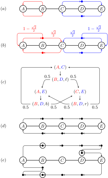
Example. We illustrate FTRV objectives and the functionality of our strategy synthesis algorithm on the graph of Fig. 1(a) with five nodes V = {A, B, C, D, E} arranged into a line where traversing each edge takes 1 time unit (this models an open perimeter with five locations at regular intervals). Even for this simple instance, our algorithm constructs solutions outperforming the best known strategies, and also rediscovers some results presented in previous works. Since these observations are important, we explain them in greater detail.
Let us first consider the problem of constructing strategies for two reliable agents (red and blue) such that the maximal expected time for visiting each node is as small as possible and both strategies are stochastically stable to a chosen degree. This is expressed by a FTRV objective 1
Here, κ ≥ 0 is a constant "punishing" the standard deviation √VT(v, 0) (a smaller deviation is enforced by a larger κ). We start with the case when κ=0, i.e., we optimize just the maximal expected time for visiting a node.
One trivial solution is to follow the aforementioned approach (A), split the nodes among the agents, and construct two trivial "cycling" strategies of Fig. 1(a). The maximal ET(v, 0) is then equal to 3, regardless of the initial agents' positions (the blue agent needs 3 time units to visit C when it is in D and moves to E in the next step). Actually, this is the best outcome achievable by any deterministic solution 2 (the existing algorithms construct only deterministic strategy profiles). However, our algorithm discovers better solutions, both in the autonomous and the coordinated case.
In the autonomous case, our algorithm computes (a rational approximation of) the solution of Fig. 1(b). Both agents use two memory states, because the decision taken in B (or D) depends on whether the red (or blue) agent came from the node on the left or right. The initial configuration is (A,Dℓ), i.e., the red agent is in A, and the blue agent is in D, behaving as if it came from C. The maximal ET(v, 0) is 1+√2 ≈ 2.41, attained for, e.g., ET(C, 0) in the configuration (A, Dℓ). Hence, this solution outperforms any deterministic solution in the expected performance. However, one can still argue that the probability of visiting C from (A,Dℓ) in 4 or more time units is positive, while the deterministic solution of Fig. 1(a) does not suffer from this deficiency.
1 The objective aims at minimizing the maximal value of the sum ET(v, 0)+κ · √VT(v, 0) over all reachable configurations, see Section 2.
2 This can be proven as follows. For the sake of contradiction, assume there is a determininistic solution s.t. the maximal ET(v, 0) is 2. Then C must be visited by some agent after k ≥ 1 time units. Hence, this agent visits nodes X,C,Y after k-1,k,k+1 time units, where X, Y ∈ {B,D}. This means that the other agent must visit both A and E in the time interval k-1,k,k+1, which is impossible.
In the coordinated case, our algorithm discovers the coordinated strategy of Fig. 1(c). The initial configuration is (A, C), and then the agents collectively move to successor configurations in the indicated way. The three shared memory states ℓ, r, b, indicate whether the left/right/both agent(s) choose the next move randomly in (B,D). Note that the agents' decisions in (B, D, b) are not independent. The maximal ET(v, 0) is equal to 2, which is optimal 3 , i.e., there is no solution such that the maximal ET(v, 0) is less than 2. Furthermore, every node is visited in at most 3 time units with probability 1 from every reachable configuration. Hence, this solution outperforms any deterministic solution in expected performance, achieving the same worst-case performance.
For κ > 0, the constructed solution in the autonomous case "trades" performance for stability, i.e., the maximal ET(v, 0) increases for increasing κ. For a sufficiently large κ, we obtain a deterministic strategy where the maximal ET(v, 0) equals 3 and the maximal VT(v, 0) is 0. In the coordinated case, we obtain the same coordinated strategy of Fig. 1(c) even for κ > 0, because this strategy is actually rather stable (the maximal VT(v, 0) is equal to 1).
All of the above solutions suffer from low resilience. If one agent fails, some nodes will not be covered at all, i.e., the maximal ET(v, 1) is ∞. To obtain a resilient solution, we use a FTRV objective
Here, we wish to minimize both the maximal ET(v, 0) and the maximal ET(v, 1). For a sufficiently large α, our algorithm produces the solution of Fig. 1(d). Both agents execute the same deterministic cycle through all nodes of length 8, and the initial configuration is (A,E). Hence, the maximal ET(v, 0) is 3, and the maximal ET(v, 1) is 7. Note that a sufficiently large α naturally leads to avoiding randomization, because the best strategy for one agent is deterministic. In this case, we obtain the same solution as existing algorithms following the aforementioned approach (B).
For three agents and objective (3), our algorithm discovers the solution of Fig. 1(e). All agents execute the same deterministic cycle of length 12. The initial configuration is indicated by the three dotted circles (two agents are initially in B, but for different memory states representing different visits to B along the cycle). The maximal ET(v, 0) is 1, and the maximal ET(v, 1) is 5. This solution closely resembles the solution for continuous time multi-agent patrolling the open perimeter designed manually in [Kawamura and Soejima, 2020]. Hence, our algorithm rediscovers the design pattern of [Kawamura and Soejima, 2020] in the discrete time setting, but for somewhat different reason. The solution of [Kawamura and Soejima, 2020] is constructed to achieve the best coverage of nodes by a deterministic solution. We aim at solution optimizing the coverage both for 0 and 1 failing agent, which for suitable α leads to a deterministic strategy prioritizing the maximal ET(v, 0) over the maximal ET(v, 1).
3 To see this, realize that when C is visited by some agent, then the other agent must be located in a node of either {A,B,C} or {C,D,E}, and hence at least two time units are needed to visit E or A, respectively.
Let us note that for certain values of α, our algorithm produces randomized solutions. For example, when α is suitably small, the solution is similar to the one obtained for the FTRV objective (2) where κ = 0, and slightly "adjusted" so that all agents visit all nodes repeatedly.
1.1 RelatedWork
Strategy synthesis for multi-agent systems is a rich research area that has been deeply studied for decades [Shoham, 2008; Wooldridge, 2009; Dixon, 2019]. The finite-horizon path planning problems for (multi-)agent systems are among the most researched subjects in mobile robotics (see, e.g., [Choset, 2005; LaValle, 2006]). Recent technological advances motivate the study of infinite-horizon path planning problems where the agents (robots, humans, software processes) perform an uninterrupted task such as persistent data-gathering [Smith et al., 2011], remote software protection [Basilico et al., 2016; Ceccato and Tonella, 2011; Collberg et al., 2012], or patrolling [Huang et al., 2019; Almeida et al., 2004; Portugal and Rocha, 2011]. Some of the classical finite-horizon planning problems, such as the vehicle routing problem or the generalized traveling salesman problem [Toth and Vigo, 2001], are solved by constructing collections of deterministic cycles that can be followed arbitrarily long. Hence, they can be seen as solutions to the corresponding infinite-horizon planing problems in situations where the underlying environment does not change.
The existing strategy synthesis techniques are mainly based on analyzing the structural properties of the underlying graph (such as splitting the graph into smaller units assigned to individual agents that are subsequently solved by special methods), constructing a uniform strategy followed by all agents, or special techniques applicable to restricted topologies such as lines or circles. Since the terrain is known, agents are cooperative, and the planning horizon is infinite, the techniques for multi-agent strategy learning (see, e.g., [Gronauer and Diepold, 2022]) have not been found particularly advantageous in this context. Our algorithm is based on differentiable programming and gradient descent, inspired by the approach used in [Klaˇska et al., 2021] for single-agent adversarial patrolling.
Randomized strategies have been used mainly in adversarial patrolling based on Stackelberg equilibria [Sinha et al., 2018; Yin et al., 2010] to reduce agents' predictability. Otherwise, randomization has been mostly avoided in infinitehorizon path planning, apparently for several reasons: randomized strategies are not apt for human agents (drivers, police squads, etc.), they are harder to construct, and their capability for delivering better performance (as demonstrated in the above example) is not immediately apparent.
Resilience to agent failures has so far been studied for (non-adversarial) surveillance and deterministic strategies. In [Hazon and Kaminka, 2005], a robust solution is obtained by constructing a cycle in the underlying graph followed by all agents with shifted initial positions. It is observed that longer cycles visiting some nodes repeatedly may improve performance (the strategy of Fig. 1(e) constructed by our algorithm has the same property). In [Czyzowicz et al., 2017], the strategy synthesis for n agents out of which precisely f are faulty is studied, again for deterministic strategies. This corresponds to the FTRV objective
However, considering deterministic strategies is insufficient for achieving optimal results (even if f = 0), as demonstrated in Fig. 1(b)(c). In particular, deterministic strategies cannot use the "entagled" randomized choice performed by the coordinated strategy of Fig. 1(c), which is crucial for decreasing the maximal ET(v, 0) to 2.
General specification languages for infinite-horizon objectives in multi-agent systems are mostly based on temporal logics (see, e.g., [van der Hoek and Wooldridge, 2012] for an overview. A formula of such a logic specifies desirable properties of trajectories, and the constructed strategies are deterministic. The idea of trading performance for stochastic stability had been studied for systems with one agent, where the underlying objectives are specified as mean payoff functions [Br´azdil et al., 2017] or recurrent reachability criteria [Klaˇska et al., 2022].
To the best of our knowledge, the results of this paper are the first attempt to solve the optimization problem for complex objective functions "balancing" the requirements on the expected time for visiting configurations, resilience, and stochastic stability of the constructed solutions for n agents. Contrasting to previous works on multi-agent strategy synthesis for infinite-horizon objectives, our algorithm computes randomized solutions (autonomous or coordinated), achieving strictly better performance than deterministic solutions produced by previous works.
2 Mathematical Model
We assume familiarity with basic notions of probability theory (expected value, variance, etc.) and Markov chain theory. A finite Markov chain is represented as a pair M = (S, Prob) where S is a finite set of states and Prob : S × S → [0, 1] is a stochastic matrix such that ∑s′∈S Prob(s, s′ ) = 1 for every s ∈ S. For a given state s and a subset F ⊆ S, we use E[Time(s→F)] to denote the expected length of a trajectory from s to a state of F , and Var[Time(s→F )] to denote the corresponding variance. A state of M is reachable if it is visited from a given initial state with positive probability. For a finite set A, we use Dist(A) to denote the set of all probability distributions over A.
2.1 Environment
The environment is modeled as a directed graph G = (V, E) where the vertices V correspond to locations visited by the agents and the edges E ⊆ V × V model admissible agents' moves between the locations. For simplicity, we assume that traversing each edge takes one time unit (general traversal times can be modeled by inserting auxiliary vertices). For the rest of this section, we fix an environment G = (V, E).
2.2 Strategies for Autonomous Agents
In the autonomous case, every agent Ai uses its private finite set Mi of memory states to store some information about the sequence of previously visited vertices. The next move of Ai is selected randomly according to the currently visited vertex and the current memory element.
More precisely, a moving strategy for Ai is a function σi : V×Mi →Dist(V×Mi). We require that whenever σi(v,m) selects (v′ ,m′ ) with positive probability, then (v, v′ ) ∈ E.
A strategy profile for agents A1, . . . ,An is a tuple σ = (σ1, . . . , σn), where every σi is a moving strategy for Ai. A configuration is a tuple [(v1,m1), . . . , (vn,mn)] describing the current vertex and the current memory state of every agent. From a given initial configuration, the agents start to execute their moving strategies simultaneously and independently. Thus, the agents proceed from one configuration to another. The next configuration is reached in one time unit, and it is selected randomly in the expected way.
More precisely, we define a Markov chain Mσ where the states are the configurations, and for all configurations c = [(v1,m1), . . . , (vn,mn)] and c′ = [(v′1 ,m′1 ), . . . , (v′n ,m′n )], we put Prob(c, c′ ) = ∏ni=1 σi(vi, mi)(v′i , m′i ).
2.3 Strategies for Fully Coordinated Agents
In the fully coordinated case, the information about the histories of agents' moves is stored in a "global" memory M consisting of finitely many states, and a coordinated strategy for n agents is a function π : V n×M → Dist(V n×M). Hence, the next move of every Ai depends on the current positions of all agents and the current state of the global memory. Here, a configuration becomes a tuple of the form (v1, . . . , vn,m), and the Markov chain Mπ over the configurations is defined in the straightforward way.
2.4 FTRVObjectives
The class of fault-tolerant recurrent visit (FTRV) objectives is built upon atoms of the form ET(v, f) and VT(v, f), where v ∈ V is a target node and f ≥ 0 is the number of faulty agents. We start by explaining the semantics of these two atoms.
Let µ be a strategy profile or a coordinated strategy for n agents where n > f (i.e., at least one agent is not faulty). For all v ∈ V and A ⊆ {A1, . . . ,An}, let C(v,A) be the set of all configurations of Mµ where at least one agent of A is located in v. Furthermore, let Reach be the set of all reachable configurations of Mµ, and let Ag[f] be the set of all A ⊆ {A1, . . . , An} such that A contains precisely n-f agents. The (µ, c,A)-value of ET(v, f), where c ∈ Reach and A ∈ Ag[f], is defined as follows:
Hence, ETµ,c,A(v, f) is the expected time for visiting target v from the configuration c by an agent of A.
Similarly, the (µ, c,A)-value of VT(v, f), denoted by VTµ,c,A(v, f), is defined as the variance of the time for visiting target v from c by an agent of A, i.e.,
A term is an expressions t built over numerical constants and atoms using differentiable functions such as multiplication or addition (each atom in t may use different v and f). The (µ, c,A)-value of t, denoted by tµ,c,A, is obtained by substituting each atom in t with its (µ, c, A)-value and evaluating the resulting expression. Furthermore, we define tµ = maxc∈Reach maxA∈Ag[f] tµ,c,A.
A FTRV objective function is an expression U of the form
where every αi is a positive weight, and every Ei is a finite set of terms. The µ-value of U, denoted by U µ , is defined as ∑mi=1 αi · max{tµ | t ∈ Ei}.
A FTRV objective is an objective of the form minimize U, where U is a FTRV objective function.
Examples
Simple examples of FTRV objectives are given in Section 1. Here we show how to express some of the unbounded-horizon path planning objectives studied for multi-agent systems in previous works.
A widely accepted effectiveness measure for deterministic strategy profiles in robotics is idleness, i.e., the maximum time between successive visits of each node. Let σ be a deterministic strategy profile achieving a finite idleness I. Then, every node of V is visited infinitely often by some agent, and the longest time elapsed between successive visits to a given v ∈ V is equal to ET(v, 0) + 1. Hence, the problem of minimizing idleness is expressible as the FTRV objective
The first summand is the idleness (the "+1" can be safely removed from all terms, because the resulting objective is equivalent), and the second summand "enforces" determinism with a suitable weight α. Since robotic agents can easily implement randomized strategies, more efficient solutions can be obtained by using objective (2), as demonstrated in Section 1.
In adversarial patrolling, a malicious attacker observes the agents and aims to initiate an attack (e.g., set a fire at a chosen node) maximizing the damage proportional to the time of discovering the attack and the vulnerability of the node. The goal is to minimize the damage caused by an optimal attack. Since the attack may be initiated right after all agents start moving to the next configuration, the worst expected time for discovering an attack at v is ET(v, 0)+1 and not just ET(v, 0). Hence, the patrolling objective can be expressed as
where wv is a constant representing the vulnerability (importance) of v. Objective (9) can be further refined by adding requirements on stochastic stability and/or resilience. Such refinements have not been studied in previous works.
Finally, let us note that the strategy profiles and coordinated strategies constructed by our synthesis algorithms are ergodic, i.e., for every µ there exists a unique limit frequency of visits to every reachable configuration c, denoted by Fµ (c). If we additionally fix a probability distribution F on Ag[f] such that F(A) is the probability that the agents of A are correct under the condition that precisely f agents are faulty, we can rigorously define the long-run average µ-value of every term t by
and enrich our language of FTRV objectives with the Avg operator. For the sake of simplicity, we keep our current setting.
3 Strategy Synthesis Algorithm
In this section, we describe our strategy synthesis algorithm for autonomous strategy profiles and coordinated strategies. In principle, these are two different algorithms, but their functionality is similar and it possible to describe both of them at
Algorithm 1 Solution synthesis
SolutionParameters ← RandomInit (V, E) for i ∈ {1, . . . , Steps} do µ ← Softmax (SolutionParameters) U µ ← Evaluate(µ) ∇U (µ) ← Gradient (µ) SolutionParameters += Step(∇U(µ)) Save U µ , µ return µ with the least U µonce. The main difference is the sets of parameters representing a strategy profile σ and a coordinated strategy π. The Markov chains Mσ and Mπ are constructed differently (see Section 2), but our algorithm processes them in the same way.
For the rest of this section, we fix a graph G = (V, E). We collectively refer to strategy profiles and coordinated strategies as solutions.
Our algorithm is based on differentiable programming and gradient descent, and it performs the standard optimization loop shown in Algorithm 1. We start by identifying a set of real-valued parameters representing a solution.
- For an autonomous strategy profile, for every agent Ai and every (v,m) ∈ V ×Mi, we need |Succ(v) ×Mi| parameters to represent the distribution σi(v,m), where Succ(v) is the set of immediate successors of v. The size of each Mi is a hyper-parameter of our algorithm.
- For a coordinated π, we need |M| · ∏ni=1 |Succ(vi)| parameters to represent the distribution π(v1, . . . , vn,m).
These parameters are initialized to random values sampled from LogUniform distribution so that we impose no prior knowledge about the solution. Then, these values are transformed into probability distributions using the standard Softmax function, obtaining the corresponding solution µ.
The crucial ingredient of Algorithm 1 is a procedure for evaluating a given FTRV objective function U for µ (see Section 3.1). This procedure allows to compute U µ , and also the gradient of U at the point corresponding to µ by automatic differentiation. After that, we update the point representing the current µ in the direction of the steepest descent. The intermediate solutions and the corresponding values of U are stored, and the best solution found within Step optimization steps is returned. Our implementation uses PYTORCH framework [Paszke et al., 2019] and its automatic differentiation with ADAM optimizer [Kingma and Ba, 2015]).
3.1 Evaluating Solutions
Let us fix a FTRV objective function U and a solution µ. Recall the definition of the Markov chain Mµ presented in Section 2. For all c, d ∈ Mµ, we use µ(c, d) to denote the probability of the transition from c to d (i.e., the value Prob(c, d), where Prob is the stochastic matrix of Mµ).
Let H be the underlying directed graph of Mµ, where the vertices are configurations, and (c, d) is an edge of H iff µ(c, d) > 0. First, we apply the Tarjan's algorithm [Tarjan, 1972] to find all bottom strongly connected components (BSCCs) of H. Note that for each BSCC B of H, the value of U is the same for all initial configurations c ∈ B. Moreover, the value of U for an initial configuration c not belonging to any BSCC cannot be lower than the value of U obtained for an initial configuration belonging to a BSCC reachable from c. Hence, it suffices to compute the value of U for each BSCC B separately, and choose the initial configuration so that it belongs to the best BSCC (observe that this BSCC can be seen as an ergodic Markov chain; this explains the remarks at the end of Section 2.4).
So, let us fix a BSCC B, a target v ∈ V , a number of faulty agents f < n, and A ⊆ {A1, . . . , An} such that |A| = n-f . For the sake of brevity, let Tc stand for Time(c→C[v, A]). We show how to compute E[Tc] and Var[Tc] for all c ∈ B.
If B ∩ C[v,A] = ∅, then E[Tc] = ∞ for all c ∈ B, and the BSCC B is disregarded, because the agents are unable to cover v. Otherwise, we create a system of linear equations over variables (Xc)c∈B. For each c ∈ B, we put
Since B is a BSCC, it follows from standard results of Markov chain theory (see, e.g. [Norris, 1998]) that this system has a unique solution, equal to (E[Tc])c∈B.
The computation of Var[Tc] is similar. We create a system of linear equations over variables (Xc)c∈B. For every c ∈ B, we have the equation
Again, this system has a unique solution, equal to (E[Tc 2 ])c∈B. Finally, we obtain that Var[Tc] = E[Tc 2 ] - (E[Tc])2 for each c ∈ B.
Having evaluated all atoms, the value of U in B is computed in the straightforward way. Since the terms may contain only differentiable functions, we can still use automatic differentiation to compute the gradient of U.
4 Experimental Results
We focused on the following questions pertaining to our algorithm: (A) whether it is able to find or approximate optimal solutions in (smaller) instances where optimality can be easily verified manually; (B) how it scales w.r.t. increasing size of the input; (C) how does the incorporation of resilience and stochastic stability into the objectives and of memory into the agent's state affect its performance and behaviour; and (D) how does it perform on graphs with various topologies.
4.1 Benchmarks
We experimented with several benchmarks. The first is the open perimeter benchmark with 5 nodes discussed in Section 1, denoted by P5. We also consider generalizations to Pk (open perimeters of length k) for increasing odd values of k to address question (B) above. The next benchmark we consider is a 4 × 4 grid in which several edges were removed in a way preserving connectedness. This creates an irregular topology through which we address question (D). We consider several graphs of this form. Finally, we consider the "triangle" ∆
benchmark. This can be seen as a closed perimeter (a circle) of length 6 with a "shortcut" in the center. The exact topologies of these graphs are given in [Klaˇska et al., 2023, Appendix A].
4.2 Experimental Setup &Metrics
The system setup was as follows: CPU: AMD Ryzen 9 3900X (12 cores); RAM: 32GB; Ubuntu 20.04.
Each experiment is parameterized by the underlying graph G, the number of agents n, the number m of memory states per agent, the variance-punishing weight κ, and the α parameter weighting the value in case of agent failure. With an exception described later, the objective is to minimize the maximum over all vertices of the graph. I.e., for a given κ and α, the objective is
We use E to denote the objective function of (11).
When κ or α are nonzero, we report not only E, but also the individual maxima of ETµ (v, 0), ETµ (v, 1), and VTµ (v, 0) for the computed strategy µ, since these quantify how well µ performs in case of agent (dis)functionality and what is its degree of stochastic stability:
Apart from these metrics, we report the average time t per single optimization step of Algorithm 1. All benchmarks were run with 600 steps. R is not reported if α is 0.
In most of the experiments we compute coordinated strategies. Experiments with independent strategies are marked with an asterisk. These experiments show that coordinated strategies perform better than uncoordinated ones and computing the latter does not yield any advantage in speed of synthesis.
For each experimental setup, we performed 5 runs with different seeds. We report the results of the run with the best ET max . The remaining details are given the extended version of this paper [Klaˇska et al., 2023, Appendix A].
4.3 Experiments and Discussion
In Experiment 1, we studied the P5 graph for which optimal values can be computed by hand (see [Klaˇska et al., 2023, Appendix B]), addressing questions (A) and (C). The setup and the results are presented in Table 1. We experimented with various levels of variance, resilience, and memory size.
The experiments demonstrate the phenomena discussed in Section 1. In particular, coordinated strategies with memory perform better than memoryless ones (line 1 vs. line 2) or uncoordinated ones (line 2 vs. line 7, where the strategy from Section 1 is found) and randomization helps, since the value is worse when randomness is penalized (line 2 vs. line 6). Also, there is a clear tradeoff between increased resilience and the "optimistic" ET max -value which assumes that all agents work correctly (lines 2-5).
| Setup | Results | |||||
|---|---|---|---|---|---|---|
| m | κ | α | ET max | √V T max | ET max R | t (s) |
| 1 | 0 | 0.00 | 2.72 | 1.30 | N/A | <0.01 |
| 3 | 0 | 0.00 | 2.00 | 1.00 | N/A | 0.02 |
| 3 | 0 | 0.10 | 2.99 | 1.80 | 8.43 | 0.02 |
| 3 | 0 | 0.50 | 3.11 | 0.94 | 6.79 | 0.02 |
| 3 | 0 | 1.00 | 3.23 | 1.00 | 6.58 | 0.02 |
| 3 | 1 | 0.00 | 3.00 | 0.00 | N/A | 0.02 |
| ∗2 | 0 | 0.00 | 2.44 | 1.16 | N/A | <0.01 |
| Setup | Results | |||
|---|---|---|---|---|
| k | κ | ET max | √V T max | t (s) |
| 7 | 0 | 4.01 | 1.97 | 0.05 |
| 7 | 1 | 5.00 | 0.00 | 0.05 |
| 9 | 0 | 5.85 | 3.06 | 0.17 |
| 9 | 1 | 7.00 | 0.00 | 0.18 |
| 11 | 0 | 7.76 | 4.47 | 0.61 |
| 11 | 1 | 9.00 | 0.00 | 0.63 |
| 13 | 0 | 9.92 | 5.02 | 1.71 |
| 13 | 1 | 11.00 | 0.00 | 1.67 |
| ∗7 | 0 | 4.21 | 1.91 | 0.07 |
| ∗9 | 0 | 5.87 | 2.97 | 0.36 |
In Experiment 2, we addressed question (B). We kept increasing the size of the open perimeter and observed the increase in runtime. We also experimented with the variance parameter to see whether the determinism/value payoff demonstrated on P5 can be observed also here. The results are presented in Table 2.
As expected, the runtime increases with graph size, although it stays well within practical limits. Penalizing randomness (even lines up to line 8) leads to deterministic strategies whose value is equivalent to the situation where the agents synchronously sweep the line as in Figure 1 (d). Allowing more randomness helps significantly. In case of P9P13, the gain in ET max is more than one, suggesting that the strategies perform more intricate behavior than simply splitting the line into 2 parts and sharing the middle node in a randomized way. Similar gain can be seen in the uncoordinated case, though it is not as large as in the coordinated one.
In Experiment 3, we analyzed two instances of the 4 × 4 grid graph with several removed edges. In G, the objective function is as described in (11). In H (which has a different topology than G), the maxima in (11) are only taken over a subset T ⊆ V of target nodes. This simulates patrolling scenarios where T are the valuable targets to protect and the remaining nodes represent transit routes etc. We experiment with various resilience parameters to analyze the tradeoff between optimal values and resilience in this scenario, addressing questions (B)-(D). The results are presented in Table 3.
| Setup | Results | |||||
|---|---|---|---|---|---|---|
| G | κ | α | ET max | √V T max | ET max R | t (s) |
| G | 0.00 | 0.10 | 13.60 | 8.38 | 27.52 | 19.58 |
| G | 0.00 | 0.00 | 11.00 | 0.00 | N/A | 6.12 |
| G | 0.10 | 0.00 | 11.00 | 3.63 | N/A | 6.11 |
| H | 0.00 | 0.10 | 11.00 | 0.00 | 23.00 | 6.00 |
| H | 0.00 | 0.00 | 10.86 | 6.12 | N/A | 2.03 |
| H | 0.10 | 0.00 | 11.00 | 0.00 | N/A | 2.04 |
| Setup | Results | ||||||
|---|---|---|---|---|---|---|---|
| G | m | κ | α | ET max | √V T max | ET max R | t (s) |
| ∆ | 2 | 0.00 | 0.00 | 2.16 | 1.11 | N/A | 3.71 |
| ∆ | 1 | 0.00 | 0.00 | 2.03 | 1.10 | N/A | 0.69 |
| P5 | 1 | 0.00 | 0.50 | 1.83 | 0.55 | 4.98 | 0.20 |
| P5 | 1 | 0.10 | 0.10 | 1.00 | 0.00 | 5.04 | 0.18 |
We can already observe a significant increase in computation time. The quality of the resulting strategy is affected by the graph topology and distribution of targets. In G, already the optimization of ET max leads to the best result and deterministic cycling through the graph. In H, there is a tradeoff between ET max and resilience, since in non-resilient case the agents are motivated to divide the target states among themselves. Again, randomization outperforms deterministic strategies (line 5 vs. line 6).
In Experiment 4, we focused on scenarios with three agents over the triangle and P5 graphs (questions (B)-(D)). In ∆, the tool found a memoryless randomized strategy whose value is close to the optimal memoryless value. On the P5 graph we see an interesting tradeoff between ET max and resilience. Already for a relatively low κ the tool finds a deterministic strategy with finite R while keeping the optimistic value ET max optimal. Further increase of κ leads to a modest improvement in resilience at the cost of a notable increase of ET max .
5 Conclusions
Our results show that optimizing complex objectives involving expected time for visiting configurations, stochastic stability, and resilience is feasible for non-trivial instances. As it was mentioned in Section 2, the class of FTRV objectives can be further enriched by operators allowing for specifying long-run average values of terms, and thus express other well-known performance measures such as average idleness.
Another challenge is to improve the overall performance of our synthesis algorithm. Since the graphs representing environments are typically sparse, using appropriate data structure might lead to a substantial speedup. Another possibility is to reduce the complexity by identifying and exploiting various types of symmetries occuring in the analysis of the Markov chain Mµ for a given solution µ.
Acknowledgments
Research was sponsored by the Army Research Office and was accomplished under Grant Number W911NF-21-1-0189. Disclaimer. The views and conclusions contained in this document are those of the authors and should not be interpreted as representing the official policies, either expressed or implied, of the Army Research Office or the U.S. Government. The U.S. Government is authorized to reproduce and distribute reprints for Government purposes notwithstanding any copyright notation herein.
Martin Kureˇcka received funding from the European Union's Horizon Europe program under the Grant Agreement No. 101087529. Petr Novotn´y is supported by the Czech Science Foundation grant GA23-06963S.
@inproceedings{ijcai2023p20,
  title     = {Synthesizing Resilient Strategies for Infinite-Horizon Objectives in Multi-Agent Systems},
  author    = {Klaska, David and Kucera, Antonin and Kurečka, Martin and Musil, Vit and Novotný, Petr and Rehak, Vojtech},
  booktitle = {Proceedings of the Thirty-Second International Joint Conference on
               Artificial Intelligence, {IJCAI-23}},
  publisher = {International Joint Conferences on Artificial Intelligence Organization},
  editor    = {Edith Elkind},
  pages     = {171--179},
  year      = {2023},
  month     = {8},
  note      = {Main Track},
  doi       = {10.24963/ijcai.2023/20},
  url       = {https://doi.org/10.24963/ijcai.2023/20},
}
TY - CPAPER TI - Synthesizing Resilient Strategies for Infinite-Horizon Objectives in Multi-Agent Systems AU - Klaska, David AU - Kucera, Antonin AU - Kurečka, Martin AU - Musil, Vit AU - Novotný, Petr AU - Rehak, Vojtech T2 - Proceedings of the Thirty-Second International Joint Conference on Artificial Intelligence, IJCAI-23 PB - International Joint Conferences on Artificial Intelligence Organization PY - 2023 SP - 171 EP - 179 DO - 10.24963/ijcai.2023/20 UR - https://doi.org/10.24963/ijcai.2023/20 ER -Copied
Machine-readable versions of this paper, for tools and AI agents:





