
An Experimental Comparison of Multiwinner Voting Rules on Approval Elections
Proceedings of the Thirty-Second International Joint Conference on Artificial Intelligence. Main Track. Pages 2675-2683.
https://doi.org/10.24963/ijcai.2023/298
Keywords
- Game Theory and Economic Paradigms: GTEP: Computational social choice
Abstract
In this paper, we experimentally compare major approval based multiwinner voting rules. To this end, we define a measure of similarity between two equal sized committees subject to a given election. Using synthetic elections coming from several distributions, we analyze how similar are the committees provided by prominent voting rules. Our results can be visualized as maps of voting rules, which provide a counterpoint to a purely axiomatic classification of voting rules. The strength of our proposed method is its independence from preimposed classifications (such as the satisfaction of concrete axioms), and that it indeed offers a much finer distinction than the current state of axiomatic analysis.
- [Aziz et al., 2017] H. Aziz, M. Brill, V. Conitzer, E. Elkind, R. Freeman, and T. Walsh. Justified representation in approval-based committee voting. Social Choice and Wel- fare, 48(2):461-485, 2017.
- [Berg, 1985] S. Berg. Paradox of voting under an urn model: The effect of homogeneity. Public Choice, 47(2):377-387, 1985.
- [Boehmer et al., 2021] N. Boehmer, R. Bredereck, P. Fal- iszewski, R. Niedermeier, and S. Szufa. Putting a compass on the map of elections. In Proceedings of IJCAI-2021, 2021. IJCAI
- [Brams et al., 2007] S. J. Brams, D. M. Kilgour, and M. R. Sanver. A minimax procedure for electing committees. Public Choice, 132(3-4):401-420, 2007.
- [Brandt and Seedig, 2013] F. Brandt and H. G. Seedig. A tournament of order 24 with two disjoint teq-retentive sets. arXiv preprint arXiv:1302.5592, 2013.
- [Brandt et al., 2013] F. Brandt, M. Chudnovsky, I. Kim, G. Liu, S. Norin, A. Scott, P. D. Seymour, and S. Thomassé. A counterexample to a conjecture of Schwartz. Social Choice and Welfare, 40(3):739-743, 2013.
- [Bredereck et al., 2019] R. Bredereck, P. Faliszewski, A. Kaczmarczyk, and R. Niedermeier. An experimental view on committees providing justified representation. In Proceedings of IJCAI-2019, pages 109-115, 2019. IJCAI
- [Brill et al., 2018] M. Brill, J.-F. Laslier, and P. Skowron. Multiwinner approval rules as apportionment methods. Journal of Theoretical Politics, 30(3):358-382, 2018.
- [Brill et al., 2023] M. Brill, R. Freeman, S. Janson, and M. Lackner. Phragmén's voting methods and justified rep- resentation. Mathematical Programming, 2023.
- [Cevallos and Stewart, 2021] A. Cevallos and A. Stewart. A verifiably secure and proportional committee election rule. In Proceedings of the 3rd ACM Conference on Advances in Financial Technologies, pages 29-42, 2021.
- [M. M. Deza and E. Deza. Encyclo- pedia of distances. Springer, fourth edition, 2016. Elkind et al., 2017] E. Elkind, P. Faliszewski, P. Skowron, and A. Slinko. Properties of multiwinner voting rules. So- cial Choice and Welfare, 48(3):599-632, 2017.
- [Enelow and Hinich, 1984] J. Enelow and M. Hinich. The Spatial Theory of Voting: An Introduction. Cambridge University Press, 1984.
- [Enelow and Hinich, 1990] J. Enelow and M. Hinich. Ad- vances in the Spatial Theory of Voting. Cambridge Uni- versity Press, 1990.
- [Faliszewski and Talmon, 2018] P. Faliszewski and N. Tal- mon. Between proportionality and diversity: Balancing district sizes under the Chamberlin-Courant rule. In Pro- ceedings of AAMAS-2018, pages 14-22, 2018.
- [Faliszewski et al., 2017a] P. Faliszewski, P. Skowron, A. Slinko, and N. Talmon. Multiwinner rules on paths from k-Borda to Chamberlin-Courant. In Proceedings of IJCAI-2017, pages 192-198, 2017. IJCAI
- [Faliszewski et al., 2017b] P. Faliszewski, P. Skowron, A. Slinko, and N. Talmon. Multiwinner voting: A new challenge for social choice theory. In Ulle Endriss, editor, Trends in Computational Social Choice, chapter 2, pages 27-47. AI Access, 2017.
- [Garey and Johnson, 1979] M. R. Garey and D. S. Johnson. Computers and Intractability: A Guide to the Theory of NP-Completeness. W. H. Freeman, 1979.
- [Gawron and Faliszewski, 2022] G. Gawron and P. Fal- iszewski. Using multiwinner voting to search for movies. In Proceedings of EUMAS-2022, pages 134-151, 2022.
- [Godziszewski et al., 2021] M. Godziszewski, P. Batko, P. Skowron, and P. Faliszewski. An analysis of approval- based committee rules for 2D-Euclidean elections. In Pro- ceedings of AAAI-2021, pages 5448-5455, 2021. [Israel and Brill, 2021]
- J. Israel and M. Brill. Dynamic pro- portional rankings. In Proceedings of IJCAI-2021, pages 261-267, 2021. IJCAI
- [Kamada and Kawai, 1989] T. Kamada and S. Kawai. An al- gorithm for drawing general undirected graphs. Informa- tion Processing Letters, 31(1):7-15, 1989.
- [Lackner and Skowron, 2021] M. Lackner and P. Skowron. Consistent approval-based multi-winner rules. Journal of Economic Theory, 192:105173, 2021.
- [Lackner and Skowron, 2023] M. Lackner and P. Skowron. Multi-Winner Voting with Approval Preferences -Artificial Intelligence, Multiagent Systems, and Cognitive Robotics. Springer Briefs in Intelligent Systems. Springer, 2023.
- [Lackner et al., 2023] M. Lackner, P. Regner, and B. Krenn. abcvoting: A Python package for approval-based multi- winner voting rules. Journal of Open Source Software, 8(81):4880, 2023.
- [Lenstra, 1983] H. W. Lenstra. Integer programming with a fixed number of variables. Mathematics of Operations Research, 8(4):538-548, 1983.
- [Lin, 2018] B. Lin. The parameterized complexity of the k- biclique problem. Journal of the ACM, 65(5):34:1-34:23, 2018.
- [Lu and Boutilier, 2011] T. Lu and C. Boutilier. Budgeted social choice: From consensus to personalized decision making. In Proceedings of IJCAI-2011, pages 280-286, 2011. IJCAI
- [McCabe-Dansted and Slinko, 2006] J. McCabe-Dansted and A. Slinko. Exploratory analysis of similarities between social choice rules. Group Decision and Negotiation, 15:77-107, 2006.
- [Peters and Skowron, 2020] D. Peters and P. Skowron. Pro- portionality and the limits of welfarism. In Proceedings of EC-2020, pages 793-794, 2020.
- [Renwick and Pilet, 2016] A. Renwick and J. B. Pilet. Faces on the Ballot: The Personalization of Electoral Systems in Europe. Oxford University Press, 2016.
- [Sánchez-Fernández et al., 2017] L. Sánchez-Fernández, E. Elkind, M. Lackner, N. Fernández, J. A. Fisteus, P. Basanta Val, and P. Skowron. Proportional justified representation. In Proceedings of AAAI-2017, pages 670-676, 2017.
- [Sapała, 2022] K. Sapała. Algorithms for embedding metrics in Euclidean spaces. Master's thesis, AGH University of Science and Technology, 2022.
- [Skowron et al., 2015] P. Skowron, P. Faliszewski, and A. Slinko. Achieving fully proportional representation: Approximability result. Artificial Intelligence, 222:67- 103, 2015.
- [Stolicki et al., 2020] D. Stolicki, S. Szufa, and N. Talmon. Pabulib: A participatory budgeting library. arXiv preprint arXiv:2012.06539, 2020.
- [Subiza and Peris, 2017] B. Subiza and J. E. Peris. A repre- sentative committee by approval balloting. Group Deci- sion and Negotiation, 26(5):1029-1040, 2017.
- [Szufa et al., 2020] S. Szufa, P. Faliszewski, P. Skowron, A. Slinko, and N. Talmon. Drawing a map of elections in the space of statistical cultures. In Proceedings of AAMAS- 2020, pages 1341-1349, 2020.
- [Szufa et al., 2022] S. Szufa, P. Faliszewski, L. Janeczko, M. Lackner, A. Slinko, K. Sornat, and N. Talmon. How to sample approval elections? In Proceedings of IJCAI- 2022, pages 496-502, 2022. IJCAI
References were extracted automatically from the PDF and may contain errors.
Full text extracted automatically from the PDF; figures, tables and equations may differ. The PDF is the version of record.
1 Introduction
Multiwinner voting is the process of selecting a fixed number of candidates (a committee) based on the preferences of agents. This general task occurs in a wide range of applications such as group recommendations [Lu and Boutilier, 2011; Gawron and Faliszewski, 2022], blockchain protocols [Cevallos and Stewart, 2021], political elections [Renwick and Pilet, 2016; Brill et al., 2018], and the design of Q&A platforms [Israel and Brill, 2021]. As it is apparent from this diverse list of applications, there is a multitude of desiderata for multiwinner voting rules and their desirability depends on the setting in which they are applied. Elkind et al. [2017] and Faliszewski et al. [2017b] suggest a classification of multiwinner voting rules based on three principles: proportionality, diversity and individual excellence. These principles capture three main goals in multiwinner voting: (i) to find a committee that reflects the voters' preferences in a proportional manner, (ii) to find a committee that represents (or, covers) the opinions of as many voters as possible (diversity), and (iii) to find a committee that contains the objectively "best" candidates (individual excellence).
In recent years, a large body of work has helped to shape our understanding of multiwinner voting rules (as surveyed by Faliszewski et al. [2017b] and Lackner and Skowron [2023]). The key method employed here is axiomatic analysis. Among the three aforementioned principles, proportionality has received the most attention and there now exists a hierarchy of proportionality axioms by which the proportionality of a voting rule can be assessed [Lackner and Skowron, 2023, Chapter 4]. Far fewer axioms exist for diversity and individual excellence [Faliszewski et al., 2017a; Subiza and Peris, 2017; Faliszewski and Talmon, 2018; Lackner and Skowron, 2021].
While the axiomatic method has been fundamental in advancing our understanding of multiwinner rules, significant questions cannot be approached with axioms. First and foremost, the satisfaction of an axiom is a binary fact. If an axiom is not satisfied by a voting rule, this might be due to a fundamental incompatibility that is evidenced in nearly every election or simply due to an involved counterexample that hardly occurs in practice (an extreme example is provided in the work of Brandt et al. [2013], which disproved an over 20year-old conjecture by giving a counterexample with 10136 candidates; however, a much smaller example was later reported by Brandt and Seedig [2013]). Secondly, while the axiomatic approach is useful to highlight differences between voting rules, it is rarely helpful to establish similarities. Even voting rules that do not share (known) axiomatic properties can behave very similarly on sampled or real-world preference data. Identifying similar voting rules is important, e.g., if a computationally demanding rule is infeasible in a given setting and has to be replaced with a faster-to-compute one.
The goal of our paper is to close this gap in our understanding and provide a principled method to assess the similarity of voting rules. Our proposed method does not rely on preimposed classifications (such as the proportionality/diversity/individual excellence trichotomy) and, instead, we base our analysis on comparing the committees provided by the rules. Specifically, given a distance measure between candidates (which we interpret as a measure of their similarity), we extend it to committees and compare how close are the committees output by a number of major multiwinner rules on several families of synthetic elections. For the visualization of our results, we adapt the map framework proposed by Szufa et al. [2020] and Boehmer et al. [2021] to display voting rules instead of elections.
Our distances between candidates depend solely on which voters approve them. For example, if two candidates are approved by the same voters, then we view them as being at distance zero, and if the voters can be partitioned into those approving either one candidate or the other, then we view these candidates as maximally distant. To measure the distance between two committees, we first build a bipartite graph with members of one committee on the left and members of the other committee on the right, where each two candidates (from the other committees) are connected by an edge whose weight is equal to their distance. The distance of the committees is the weight of the minimum-weight perfect matching in this graph. Our main findings are as follows:
- We show that computing two most distant committees in a given election is intractable in many settings. This is somewhat unfortunate, as such committees would be useful to normalize the distances between committees. Due to this hardness result, in the remainder of the paper we normalize by observed maximum distances.
- We compute the committees output by various multiwinner rules on a number of synthetic elections and compute the average distances between committees provided by different rules. We find that committees provided by Multiwinner Approval Voting (AV), ChamberlinCourant (CC), and Minimax Approval Voting tend to be the most distinct ones, while those provided by proportional rules are between those of AV and CC (often, but not always, closer to AV), and far away from those of Minimax.
- For a number of proportionality axioms, we report how often the committees output by various rules satisfy them. Surprisingly, our experiments show that the committees provided by proportional voting rules (on sampled profiles) generally satisfy stronger proportionality properties than their axiomatic analysis reveals. In particular, we find that some axiomatic distinctions are not observable in our data set of 6000 instances.
All in all, we find that all proportional rules-including those that fail some of the stronger proportionality axioms-are more or less similar to each other and form a well-defined cluster.
2 Preliminaries
For a given graph G = (V (G),E(G)) and a vertex x ∈ V (G), by N(x) we denote the neighbors of x (i.e., the set {y ∈ V (G) : (x, y) ∈ E(G)}) and by deg(x) we denote the degree of x (i.e., deg(x) = |N(x)|).
2.1 Elections
We consider the approval preference model. An election E = (C, V ) consists of a set C = {c1, . . . , cm} of candidates and a collection V = (v1, . . . , vn) of voters, where each voter vi is endowed with a set of candidates that they approve. For a voter v we denote his or her approval set as A(v), and for a candidate c we write A(c) to denote the set of voters that approve c. Whenever we use this notation, the election in question will be clear from the context.
2.2 Multiwinner Voting Rules
An approval-based multiwinner voting rule is a function f that given an election E = (C, V ) and committee size k, k ≤ |C|, provides a family f(E, k) of size-k subsets of C, referred to as the winning committees.
We give a brief overview of major approval-based multiwinner voting rule. We omit technical details and refer to the survey by Lackner and Skowron [2023] for details. We assume that all voting rules use a tiebreaking mechanism to ensure that they return exactly one winning committee (this property is known as resoluteness). 1
Thiele methods are an important class of approval-based multiwinner voting rules that select a committee W maximizing value scw(W) = ∑v∈V ∑|A(v)∩W| i=1 w(i) for some score function w. In particular, Multiwinner Approval Voting (AV) is defined by w(i) = i (equivalently, AV selects the k candidates that are approved by the largest number of voters). This rule is considered to be the prime example of the principle of individual excellence. ChamberlinCourant (CC) selects the committee W that maximizes the number of voters that approve at least one candidate in W, i.e., w(1) = 1 and w(i) = 0 for all i ̸= 1. CC is an example of a rule designed to achieve diversity. Proportional Approval Voting (PAV) and Sainte-Lagu¨e Approval Voting (SLAV) are defined by w(i) = 1i and w(i) = 1 2i-1 , respectively. Finally, p-Geometric rules are defined by w(i) = p-i for positive constants p. The weights of PAV can be viewed as the most proportional choice in this spectrum [Aziz et al., 2017; S´anchez-Fern´andez et al., 2017]; weight functions that decrease more quickly than that of PAV (such as those used by SLAV and p-Geometric rules) give more importance to small groups (degressive proportionality).
Sequential Thiele methods, also referred to as greedy Thiele rules in the literature, iteratively build a committee by adding the candidate that increases the score scw most, starting with the empty committee and iterating until k candidates are selected. We consider seq-PAV, seq-SLAV, and seq-CC. Greedy Monroe [Skowron et al., 2015] is a rule similar to seqCC, with an additional constraint that each committee member can represent at most n/k many voters.
Satisfaction Approval Voting (SAV) is defined similarly to AV and selects a committee W maximizing ∑v∈V |A(v)∩W | |A(v)| . Minimax Approval Voting (MAV) [Brams et al., 2007] selects a committee W that minimizes maxv∈V |A(v) \ W| + |W \ A(v)|, i.e., it minimizes the maximumHamming distance between a voter and the chosen committee.
Finally, we describe the intuition behind two slightly more complex rules: Sequential Phragm´en (seq-Phragm´en) [Brill et al., 2023] and the method of Equal Shares [Peters and Skowron, 2020]. Both can be understood as mechanisms where voters use (virtual) budget to jointly pay for the selection of candidates in the committee. The cost of adding a candidate is set (arbitrarily) to 1. With seq-Phragm´en, voters start with a budget of 0, which is increased continuously until a group of voters can pay for the first candidate. The cost (of 1) is shared among the members of the group and the process repeats until the committee is filled. With Equal Shares, voters start with a budget of k/n. Each round, a candidate is selected that requires the least budget per voter. This procedure may result in fewer than k committee members (since the budget is fixed in advance), in which case seq-Phragm´en is used to fill the committee. We refer to the works of Lackner et al. [2023] and Peters and Skowron [2020] for details.
1 On the technical level, in our experiments we use the implementations of the rules provided in the abcvoting library [Lackner et al., 2023], together with their default tie-breaking.
2.3 Proportionality
Much of the recent progress in multiwinner voting has been dedicated to the concept of proportionality, to formally define proportionality and to identify voting rules behaving proportionally. Since our framework enables us to identify similar voting rules, we are able to ask whether "proportional" rules are indeed similar. To this end, we consider four proportionality axioms. These axioms apply to committees and a voting rule is said to satisfy such a property if it is guaranteed to return committees exhibiting this property.
Definition 1 (S´anchez-Fern´andez et al. 2017). Given an election E = (C, V ), a committee W of size k satisfies Proportional Justified Representation (PJR) if there is no group of agents N ⊆ V of size |N| ≥ ℓ · nk that jointly approves at least ℓ common candidates and ∣∣⋃v∈N A(v) ∩W ∣∣ < ℓ.
PJR is satisfied by PAV, seq-Phragm´en, Equal Shares, and Greedy Monroe 2 (among the rules introduced in Section 2.2).
Definition 2 (Aziz et al. 2017). Given an election E = (C, V ), a committee W of size k satisfies Extended Justified Representation (EJR) if there is no group of agents N ⊆ V of size |N| ≥ ℓ · nk that jointly approves at least ℓ common candidates and for each voter v ∈ N, |A(v) ∩W| < ℓ.
EJR strengthens PJR and is satisfied only by PAV and Equal Shares. Finally, Justified Representation (JR) is the special case of PJR (and EJR) restricted to ℓ = 1.
Priceability [Peters and Skowron, 2020] is a notion of proportionality based on assigning budget to voters.
Definition 3. Given an election E = (C, V ), a committee W satisfies priceability if there is a budget b ≥ 0 and for each voter vi a spending function bi : C → R≥0 such that:
- for each vi ∈ V , ∑c∈C bi(c) ≤ b (voters do not spend more than b),
- for each vi ∈ V , if c /∈ A(vi) then bi(c) = 0 (voters do not pay for candidates they do not approve),
- if c ∈W then ∑vi∈V bi(c) = 1 and otherwise this value is 0 (payments only for committee members), and
- for each c /∈ W, ∑vi∈A(c) (b - ∑c′∈W bi(c′ )) ≤ 1 (there is no candidate left that could be bought with more than a budget of 1).
Priceability establishes fairness by distributing the same amount of budget to each voter and requiring that no candidate could be bought with a smaller amount (condition 4). Priceability implies PJR and is incomparable to EJR. It is satisfied by seq-Phragm´en and Equal Shares.
2 It satisfies PJR if k divides n [S´anchez-Fern´andez et al., 2017].
2.4 Statistical Cultures
Below, we define the statistical cultures that we use for generating synthetic instances of approval elections.
ResamplingModel. The resamplingmodel is parameterized by two values, p ∈ [0, 1] and ϕ ∈ [0, 1], where the first one describes the average number of approvals in a vote, and the second one describes the level of disturbance. To generate an election, we first sample a central ballot by approving uniformly at random ⌊pm⌋ candidates. Then, to generate a vote, we proceed as follows. For each candidate in the central ballot, we add him or her to the vote with probability 1-ϕ, and with probability ϕ we resample that candidate, that is, we add him or her to the ballot with probability p. For each candidate outside the central ballot, with probability 1 - ϕ, we keep him or her outside the ballot, and with probability ϕ we resample him or her.
Disjoint Model. The disjoint model has three parameters, p ∈ [0, 1], ϕ ∈ [0, 1], and g ∈ N\{0}. It is similar to the resampling model, but instead of a single central ballot we have g central ballots. At the beginning, we sample g disjoint central ballots uniformly at random (each of them approving ⌊pm⌋ candidates, and then proceed in the same manner as before, however before generating each vote, we uniformly at random select one of our g central ballots on which our vote will be based.
EuclideanModels. The Euclidean model is parameterized by a radius r ∈ R+. For each voter and each candidate we sample their ideal point in the t-dimensional Euclidean space (uniform in a t-dimensional cube). Then, each voter approves all the candidates within radius r.
Party-list Model. The party-list model is parameterized by α and g. First, we divide the candidates into g groups of size ⌊m/g⌋ each; we refer to these groups as the parties. (If m mod g ̸= 0 then some candidates remain unapproved.) Second, we create an urn which contains a single vote for each party, approving exactly its members. Then, we iteratively generate votes (one at a time): We draw a vote from the urn, add its copy to the election, and return the vote to the urn together with αg copies.
PabulibModel. We also use real-life participatory budgeting (PB) data from Pabulib [Stolicki et al., 2020], which we treat as a statistical culture over approval elections (in particular, we omit details related to PB, such as the costs of the candidates). We selected 21 instances, i.e., all that contain at least 100 candidates and 100 voters, and where the average number of approved candidates per voter is at least 3 (for instances with truncated ordinal ballots, we convert them to approval ones by approving all candidates that were ranked). To sample an election from Pabulib, we first uniformly at random choose one of the original 21 instances, then we randomly select a subset of 100 candidates and a random subset of 100 voters. We omit voters who cast empty ballots.
The resampling and disjoint models are due to Szufa et al. [2022]. Various Euclidean models are commonly used in the literature on elections [Enelow and Hinich, 1984;
Enelow and Hinich, 1990]; we point to the recent works of Bredereck et al. [2019] and Godziszewski et al. [2021], which use them in the approval setting. The party-list model is an adaptation of the Polya-Eggenberger urn model [Berg, 1985; McCabe-Dansted and Slinko, 2006].
3 Similarity Between Committees
Our idea of comparing voting rules is based on measuring the similarity between the committees that they produce.
3.1 Basic Framework
Fix some election E = (C, V ) with candidate set C = {c1, . . . , cm} and voter collection V = (v1, . . . , vn). We assume that we have some distance d over the candidates, such that if d(ci, cj) is small-for whatever "small" means under a given distance-then candidates ci and cj are similar, and if it is large then they are not. In the most basic setting we could take the discrete distance, where disc(ci, cj) = 0 exactly if i = j and disc(ci, cj) = 1 for every other case. Later we will discuss two more distances.
Let X = {x1, . . . , xk} and Y = {y1, . . . , yk} be two sizek committees over C. We extend d to act on committees as follows: We form a bipartite graph with members of X as the vertices on the left, members of Y as the vertices on the right, and where for each x ∈ X and each y ∈ Y we have an edge with weight d(x, y); if some candidate c belongs to both X and Y , then we have two copies of c, one on the left and one on the right. The distance d(X, Y ) between X and Y is the weight of the minimum-weight matching in this graph. One can verify that it indeed is a pseudodistance.
Proposition 1. For each (pseudo)distance d over the candidates, its above-described extension to committees is a pseudodistance.
Proof. Let X = {x1, . . . , xk}, Y = {y1, . . . , yk}, and Z = {z1, . . . , zk} be three size-k committees from the same election. By definition of d, we immediately get that d(X,X) = 0 and d(X, Y ) = d(Y,X). It remains to show that d(X, Y ) ≤ d(X, Z) + d(Z, X). By reordering the members of X, Y , and Z, we can assume that:
Since d is a distance, for each i ∈ [k] we have d(xi, yi) ≤ d(xi, zi) + d(zi, yi). Further, we know that d(X, Y ) ≤ d(x1, yi) + · · · + d(xk, yk) (because instead of using the lowest-weight matching we use some fixed one). By putting these inequalities together, we get that, indeed, d(X, Y ) ≤ d(X, Z) + d(Z, Y ).
Let us now consider concrete distance measures between candidates, all of which are well-known distances (cf. [Deza and Deza, 2016]). The discrete distance is a rather radical approach as it stipulates that no two candidates are ever similar to each other. Yet, one could argue that there are cases where some candidates are clearly more similar to each other than others.
Example 1. Consider an election E = (C, V ) with C = {p, q, r, s} and voter collection V = {v1, v2, v3, v4). The approval sets are as follows:
One could argue that candidates p and q are completely dissimilar because they are approved by complementary sets of voters. On the other hand, half of the voters who approve p also approve r, and every voter who approves r also approves p. The similarity between p and s seems a bit weaker than that between p and r because there is a voter who approves s but does not approve p.
In addition to the discrete one, we consider the following two distances between the candidates (we assume some election E with n voters):
- The Hamming distance between candidates c and d, denoted by ham(c, d), is the number of voters that approve one of them but not the other. Formally, we have ham(c, d) = |A(c) \ A(d)| + |A(d) \ A(c)|.
- The Jaccard distance between candidates c and d is defined as jac(c, d) = 1 - |A(c)∩A(d)| |A(c)∪A(d)| = ham(c,d) |A(c)∪A(d)| .
There are two main differences between the Hamming and the Jaccard distances. The less important one is that the former is not normalized and can assume values between 0 and n, whereas the latter always assumes values between 0 and 1. Occasionally, we will speak of normalized Hamming distance nham(c, d) = 1/n · ham(c, d).
The more important difference is in how both distances interpret lack of an approval for a candidate. Under the Hamming distance, we assume that it is a conscious decision, indicating that a voter disapproves of a candidate. Hence, if neither candidate c nor d is approved by a voter, then Hamming distance interprets it as a sign of similarity between them. 3 Under the Jaccard distance, we assume that we cannot make any such conclusions.
Example 2. Let us consider the election from Example 1. We have the following normalized Hamming and Jaccard distances between the candidates:
As our intuition from Example 1 suggested, both our distances indicate that candidate p is completely dissimilar from candidate q, and is more similar to r than to s. However, according to the normalized Hamming distance q and r are not completely dissimilar, whereas they are at maximum distance according to Jaccard.
3 Yet, a voter might dislike c and d for two different reasonse.g., one is too liberal and the other is not liberal enough, which makes this approach questionable.
3.2 Hardness of Finding Farthest Committees
Given an election and a committee size, it is convenient to know what is the largest possible distance between two committees. In particular, one could use this value to normalize distances between committees provided by various rules. Unfortunately, it turns out that finding two farthest committees under a given distance is often intractable and in our experiments we will resort to normalizing by largest observed distances. We define the FARTHEST COMMITTEES problem as follows.
Definition 4. In the FARTHEST COMMITTEES problem (FC) we are given an election (C, V ), an integer k, and a pseudodistance d over the candidates. The goal is to output two committees, each of size k, which maximize the distance d between them.
FC can be considered also in its decision variant, where we ask if there are two size-k committees whose distance is at least a given value.
FC under the discrete distance is trivially polynomial-time solvable. In Theorem 1 we show that FC is computationally hard in the cases of the Hamming distance and the Jaccard distance. This comes through a reduction from the BALANCED BICLIQUE problem defined as follows.
Definition 5. In the BALANCED BICLIQUE problem (BB) we are given a bipartite graph G = (AG ∪ BG,EG) and an integer kG. The question is whether there exists a biclique of size kG × kG in G (kG-biclique), i.e., a set of vertices X ∪ Y such that X ⊆ AG, Y ⊆ BG, |X| = |Y | = kG and for every x ∈ X, y ∈ Y we have (x, y) ∈ EG.
BB is known to be NP-hard [Garey and Johnson, 1979, p. 196] and W[1]-hard w.r.t. kG [Lin, 2018].
The idea of the reduction is to encode vertices by candidates and edges by large distances (no-edges are represented by slightly smaller distances). A technical issue is to define proper votes in order to: 1) achieve required relation between the distances and, 2) forbid taking candidates to one committee that come from both parts of the input bipartite graph.
Theorem 1. FARTHEST COMMITTEES is NP-hard and W[1]-hard w.r.t. k (the size of committees), even in the case of the Hamming distance or the Jaccard distance.
Proof. First we show the theorem for the Jaccard distance. The reduction is from BALANCED BICLIQUE (BB). We take an instance (G = (AG∪BG, EG), kG) of BB and produce an instance of the decision version of FARTHEST COMMITTEES (FC) with the Jaccard distance.
For every vertex x ∈ AG ∪ BG we define a candidate x ∈ C. Thus, |C| = |AG ∪BG|. We overload the notation and by x we mean both a vertex x from the graph G and a candidate x from C. This is due to the bijection between them.
We define the votes as follows. There is one voter vA with an approval set AG and one voter vB with an approval set BG. Then, for every x ∈ AG we define a voter vx with an approval set {x} ∪ (BG \ N(x)) (recall that N(x) means the neighbors of x). Hence, we have |V | = |AG| + 2.
We ask for an existence of two committees of size k = kG with the Jaccard distance equal to k (indeed, k is the largest possible Jaccard distance between two size-k committees).
In order to show correctness of the reduction, it suffices to prove the following lemma which implies that only kbicliques correspond to committees at Jaccard distance k.
Lemma 1. For every X, Y ⊆ AG ∪BG, |X| = |Y | = k, the following equivalence holds: (X, Y ) is a k-biclique in G if and only if jac(X, Y ) = k.
The proof is available in the full version of the paper.
It is straightforward to see that the reduction runs in polynomial time. Hence, NP-hardness of FC follows from NPhardness of BB [Garey and Johnson, 1979, p. 196]. Furthermore, BB is W[1]-hard w.r.t. kG [Lin, 2018] and we have k = kG, so indeed, FC is W[1]-hard w.r.t. k.
In the case of the Hamming distance we use the same reduction with the following changes: (1) Instead of one voter vA we add |AG| many voters vA; (2) Instead of one voter vB we add |AG| many voters vB; (3) We add |AG| many degree-correcting voters who do not approve any candidates from AG but, for every candidate y ∈ BG, exactly deg(y) many of them approve y; (4) We ask for an existence of two committees of size k with the Hamming distance equal to k · (3|AG| + 1). After such modifications we still have C = AG ∪ BG, but we have |V | = 4 · |AG|.
In order to show correctness of the reduction it is enough to prove the following lemma.
Lemma 2. For every X, Y ⊆ AG ∪ BG, |X| = |Y | = k, the following equivalence holds: (X, Y ) is a biclique of size k × k in G if and only if ham(X, Y ) = k · (3|AG| + 1).
The proof is available in the full version of the paper.
FC with the normalized Hamming distance is also NP-hard because its objective function is just scaled compared to the Hamming distance.
Parameterized Hardness
A brute-force algorithm for FARTHEST COMMITTEES (for any distance measure) runs in time m2k · poly(n,m) (by evaluating all possible pairs of k-sized committees). Unfortunately, we cannot hope for large improvements over this as stated below.
Proposition 2. Under a randomized version of the Exponential Time Hypothesis, there is no (n+m)o(√k) -time algorithm for FARTHEST COMMITTEES. This holds even for the Hamming distance and for the Jaccard distance.
Proof. The result follows from hardness of BALANCED BICLIQUE [Lin, 2018], which excludes (under the same hypothesis) existence of |VG|o(√k) -time algorithm. Using our reduction from Theorem 1 and the fact that n = O(|VG|), m = O(|VG|), the theorem follows.
Naturally, FC is FPT w.r.t. m (for any distance measure) by a brute-force algorithm which evaluates (mk )2 ≤ 4m many pairs of committees.
Next, we show that FC is FPT w.r.t. n + k, although the dependence on a parameter is double-exponential.
| Rule | Resampling | Disjoint | Party-list | 1D | 2D | Pabulib | ||||||||||||||||||
|---|---|---|---|---|---|---|---|---|---|---|---|---|---|---|---|---|---|---|---|---|---|---|---|---|
| Equal Shares | 1.0 | 1.0 | 1.0 | 1.0 | 1.0 | 1.0 | 1.0 | 1.0 | 1.0 | 1.0 | 1.0 | 1.0 | 1.0 | 1.0 | 1.0 | 1.0 | 1.0 | 1.0 | 1.0 | 1.0 | 1.0 1.0 | 1.0 | 1.0 | |
| seq-Phragm´en | 1.0 | 1.0 | 1.0 | 1.0 | 1.0 | 1.0 | 1.0 | 1.0 | 1.0 | 1.0 | 1.0 | 1.0 | 1.0 | 1.0 | 1.0 | 1.0 | 1.0 | 1.0 | 1.0 | 1.0 | 1.0 1.0 | 1.0 | 1.0 | |
| PAV | 1.0 | 1.0 | 1.0 | 1.0 | 1.0 | 1.0 | 1.0 | 1.0 | 1.0 | 1.0 | 1.0 | 1.0 | 1.0 | 1.0 | 1.0 | 1.0 | 1.0 | 1.0 | 1.0 | 1.0 | 1.0 1.0 | 1.0 | 1.0 | |
| seq-PAV | 1.0 | 1.0 | 1.0 | 1.0 | 1.0 | 1.0 | 1.0 | 1.0 | 1.0 | 1.0 | 1.0 | 1.0 | 1.0 | 1.0 | 1.0 | 1.0 | 1.0 | 1.0 | 1.0 | 1.0 | 1.0 | 1.0 | 1.0 | 1.0 |
| SLAV | 1.0 | 1.0 | 1.0 | 1.0 | 0.95 | 1.0 | 1.0 | 1.0 | 0.36 | 1.0 | 1.0 | 1.0 | 0.88 | 1.0 | 1.0 | 1.0 | 0.99 | 1.0 | 1.0 | 1.0 | 1.0 | 1.0 | 1.0 | 1.0 |
| seq-SLAV | 1.0 | 1.0 | 1.0 | 1.0 | 0.95 | 1.0 | 1.0 | 1.0 | 0.36 | 1.0 | 1.0 | 1.0 | 0.86 | 1.0 | 1.0 | 1.0 | 0.99 | 1.0 | 1.0 | 1.0 | 1.0 | 1.0 | 1.0 | 1.0 |
| Greedy Monroe | 1.0 | 1.0 | 1.0 | 1.0 | 0.88 | 1.0 | 1.0 | 1.0 | 0.29 | 1.0 | 1.0 | 1.0 | 0.78 | 1.0 | 1.0 | 1.0 | 0.93 | 1.0 | 1.0 | 1.0 | 0.95 | 1.0 | 1.0 | 1.0 |
| Geom. 2 | 1.0 | 1.0 | 1.0 | 1.0 | 0.95 | 1.0 | 1.0 | 1.0 | 0.14 | 0.55 | 0.55 | 1.0 | 1.0 | 1.0 | 1.0 | 1.0 | 1.0 | 1.0 | 1.0 | 1.0 1.0 | 1.0 | 1.0 | 1.0 | |
| Geom. 3 | 0.99 | 1.0 | 1.0 | 1.0 | 0.87 | 0.99 | 0.99 | 1.0 | 0.03 | 0.3 | 0.3 | 1.0 | 0.88 | 1.0 | 1.0 | 1.0 | 0.99 | 1.0 | 1.0 | 1.0 | 0.97 | 1.0 | 1.0 | 1.0 |
| Geom. 4 | 0.96 | 1.0 | 1.0 | 1.0 | 0.82 | 0.98 | 0.98 | 1.0 | 0.02 | 0.23 | 0.23 | 1.0 | 0.77 | 1.0 | 1.0 | 1.0 | 0.96 | 1.0 | 1.0 | 1.0 0.93 | 1.0 | 1.0 | 1.0 | |
| Geom. 5 | 0.93 | 1.0 | 1.0 | 1.0 | 0.79 | 0.98 | 0.98 | 1.0 | 0.01 | 0.2 | 0.2 | 1.0 | 0.68 | 1.0 | 1.0 | 1.0 | 0.93 | 1.0 | 1.0 | 1.0 | 0.88 | 1.0 | 1.0 | 1.0 |
| SAV | 1.0 | 1.0 | 1.0 | 1.0 | 0.5 | 0.64 | 0.64 | 0.64 | 0.06 | 0.08 | 0.08 | 0.08 | 0.0 | 0.01 | 0.01 | 0.01 | 0.0 | 0.06 | 0.06 | 0.06 | 0.84 | 1.0 | 1.0 | 1.0 |
| AV | 1.0 | 1.0 | 1.0 | 1.0 | 0.49 | 0.63 | 0.63 | 0.63 | 0.06 | 0.08 | 0.08 | 0.08 | 0.0 | 0.01 | 0.01 | 0.01 | 0.01 | 0.12 | 0.12 | 0.12 | 0.91 | 0.98 | 0.98 | 0.98 |
| Minimax AV | 0.71 | 0.99 | 0.99 | 0.99 | 0.46 | 0.89 | 0.89 | 0.98 | 0.0 | 0.05 | 0.05 | 1.0 | 0.0 | 0.09 | 0.09 | 0.09 | 0.02 | 0.28 | 0.28 | 0.28 | 0.59 | 0.86 | 0.86 | 0.86 |
| seq-CC | 0.97 | 1.0 | 1.0 | 1.0 | 0.62 | 0.88 | 0.88 | 1.0 | 0.0 | 0.06 | 0.06 | 1.0 | 0.23 | 0.99 | 0.99 | 1.0 | 0.47 | 0.99 | 0.99 | 1.0 | 0.58 | 1.0 | 1.0 | 1.0 |
| CC | 0.21 | 0.61 | 0.65 | 1.0 | 0.62 | 0.85 | 0.86 | 1.0 | 0.0 | 0.04 | 0.04 | 1.0 | 0.23 | 0.98 | 0.99 | 1.0 | 0.42 | 0.98 | 0.99 | 1.0 | 0.56 | 1.0 | 1.0 | 1.0 |
Theorem 2. For a given candidate pseudodistance function d(x, y), which is a function of A(x) and A(y) only, FARTHEST COMMITTEES under d is FPT w.r.t. n + k.
Proof. We say that two candidates x, y have the same type if they are approved by the same voters, i.e., A(x) = A(y). Let us denote the number of candidate types by t. Clearly, we have t ≤ 2n . We find a solution by guessing how many candidates of every type are in both committees. For one committee there are at most kt ≤ k2n many choices. Hence, we can find a solution after k2n+1 many checks, each in polynomial time (by computing the minimum-weight matching).
Using more involved arguments we show that FC is FPT w.r.t. n. Such algorithm can be useful in the case when the committee size k is much larger than n.
Theorem 3. For a given candidate pseudodistance function d(x, y), which is a function of A(x) and A(y) only, FARTHEST COMMITTEES under d is FPT w.r.t. n.
The proof is available in the full version of the paper. The main technique used to provide this result is formulating FC as an Integer Linear Program (ILP) with the number of integer variables and the number of constraints being a function of n. Then, it is enough to apply the result of Lenstra [1983] for solving ILPs. The main idea for the ILP is to consider types of candidates-defined for every candidate c as a subset of voters that approve c, i.e., A(c). There are at most 2n types of candidates. Notice that two candidates of the same type have exactly the same distances to any other candidate. Hence, for each candidate type, by two integer variables we encode how many candidates of this type are included in both committees. Then, the objective function is to maximize the weight of a b-matching (a matching in which a vertex can be matched multiple times) according to the capacities defined by the integer variables. The main technical issue we faced is ensuring that the achieved matching of maximum weight is also the minimum-weight matching among the chosen candidates. We overcome this obstacle by adding 25n constraints (one for every cycle in a bipartite graph in which vertices represent types of candidates).
4 Map of Rules
In this section, we present our Map of Multiwinner Voting Rules. The map is constructed in the following way. First, we generate a number of elections from several statistical cultures (details are described later in the text). Second, we compute winning committees under the considered voting rules. We impose resoluteness, i.e., each rule outputs exactly one winning committee. Third, we compute the distances between winning committees using the Jaccard distance (we chose it over Hamming due to the way it interprets the lack of an approval for a candidate). For each election, we normalize the Jaccard distance by dividing it by the largest distance between two committees, outputted by our voting rules, for that election. For each two rules and each statistical culture, we compute the average distance between the rules' committees; this gives us distance matrices for the cultures. We embed these matrices in 2D-Euclidean space using a variant of the algorithm of Kamada and Kawai [1989], as implemented by Sapała [2022]. If two rules output similar winning committees, then we view these two rules as similar; the algorithm places such rules close to one another on the map. 4 While different runs of the algorithm (on the same distance data) may give somewhat different maps, the outputs tend to be similar, and we believe that the maps give good intuitions regarding the relative distances between the rules.
4.1 Experimental Setup
We generated 6000 instances with 100 candidates and 100 voters from the six following statistical cultures (1000 elections per culture): 1D-Euclidean with r = 0.05, 2DEuclidean with r = 0.2, resampling with p = 0.1 and ϕ ∈ {0, 1 999 , 2 999 , . . . , 998 999 , 1}, disjoint with p = 0.1, ϕ ∈ {0, 1 999 , 2 999 , . . . , 998 999 , 1}, and g = 10, party-list with g = 10, and the Pabulib model. For all instances, we use a committee size of k = 10.
4.2 Experimental Results
Results for priceability, EJR, PJR, and JR are presented in Table 1. Even though only Equal Shares and seq-Phragm´en formally satisfy priceability, for all instances that we generated, the committees provided by PAV and seq-PAV also satisfied priceability. Moreover, seq-Phragm´en and seq-PAV satisfy EJR on all instances despite seq-Phragm´en only guaranteeing PJR [Brill et al., 2023] and seq-PAV not even JR [Aziz et al., 2017]. These results indicate that instances witnessing that, e.g., seq-PAV fails EJR are rare. In turn, we can conclude that rules such as seq-PAV have stronger proportionality properties than their axiomatic analysis reveals.
Let us briefly discuss the existence of cohesive groups in our data, i.e., groups N ⊆ V with |N| ≥ ℓ · nk that jointly approves at least ℓ common candidates. If, for some reason, our data did not contain cohesive groups for ℓ ≥ 2, then the notions of EJR, PJR and JR would coincide; this would render this comparison meaningless. However, this is not the case. For example, for the Disjoint model, 311 of 1000 instances have cohesive groups with ℓ = 2; for the Resampling model this holds for 717 of 1000 instances. Further, for some models, one can see that JR is significantly easier to satisfy than, say, EJR. This is particularly apparent for CC, which is guaranteed to satisfy JR but fails both PJR and EJR. Finally, we note that our results also support the conclusion by Bredereck et al. [2019] that-under many statistical culturescommittees satisfying JR often also satisfy PJR and EJR.
4 The code for the experiments is available at https://github.com/ Project-PRAGMA/Map-of-Rules-IJCAI-2023.
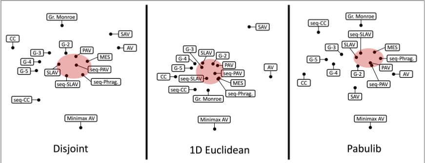
For three of our models, that is, disjoint, 1D-Euclidean, and Pabulib, we present maps of multiwinner voting rules; see Figure 1 (each map is based on 1000 elections generated for the respective culture). We start by analyzing the left map for the disjoint model. On the "west" side of the map, we have the CC voting rule; this area can be interpreted as representing diversity: the rules located in this area select committees that consist of diverse candidates. On the "east" side of the map we have AV; this area can be interpreted as representing individual excellence: the rules located here select committees that consist of individually best candidates, not taking into account whether the selected candidates are similar to each other or not. In the central part of the map (highlighted in red), we have numerous rules considered to be proportional, such as the PAV rule or seq-Phragm´en. Note that Geometric rules are close to the "cluster" of proportional rules, but their distance increases for larger p-values. Finally, in the "south" area we have Minimax AV, which is different from all the other rules. Importantly, this separation of diverse, proportional and individually excellent rules arises naturally in our model.
As for the central map, which is based on 1D-Euclidean elections, the overall location of the rules is similar. However, the "proportional cluster" is shifted toward CC. Moreover, SAV is more different from AV than in the previous map. As 1D Euclidean is a simpler model, we generally see fewer details in this map.
Finally, consider the map based on real-life elections from Pabulib. Here, we see more pronounced differences (as in the disjoint model). Interestingly, PAV and seq-PAV are almost indistinguishable here. Generally, it can be observed that the relative position of voting rules does not vary greatly across different probability models. In particular, the proportional cluster can be observed in all maps.
5 Summary
We introduced a framework for comparing multiwinner voting rules based on the committees they select. This framework gives a principled approach to identifying similarity of voting rules. When contrasted with axiomatic analysis, we see that some rules (seq-Phragm´en and seq-PAV) are not only close to strongly proportional rules (Equal Shares and PAV), but are also indistinguishable from an axiomatic point of view in our dataset. This indicates that our distance-based approach indeed offers a finer view of multiwinner rules, and thus complements a precise axiomatic analysis.
Acknowledgements
Martin Lackner was supported by the Austrian Science Fund (FWF), research grant P31890. Krzysztof Sornat was supported by the SNSF Grant 200021 200731/1. We thank Jannik Peters for helpful feedback and Pasin Manurangsi for a discussion on the hardness of the BALANCED BICLIQUE problem. This project has received funding from the European Research Council (ERC) under the European Union's Horizon 2020 research and innovation programme (grant agreement No 101002854).


@inproceedings{ijcai2023p298,
  title     = {An Experimental Comparison of Multiwinner Voting Rules on Approval Elections},
  author    = {Faliszewski, Piotr and Lackner, Martin and Sornat, Krzysztof and Szufa, Stanisław},
  booktitle = {Proceedings of the Thirty-Second International Joint Conference on
               Artificial Intelligence, {IJCAI-23}},
  publisher = {International Joint Conferences on Artificial Intelligence Organization},
  editor    = {Edith Elkind},
  pages     = {2675--2683},
  year      = {2023},
  month     = {8},
  note      = {Main Track},
  doi       = {10.24963/ijcai.2023/298},
  url       = {https://doi.org/10.24963/ijcai.2023/298},
}
TY - CPAPER TI - An Experimental Comparison of Multiwinner Voting Rules on Approval Elections AU - Faliszewski, Piotr AU - Lackner, Martin AU - Sornat, Krzysztof AU - Szufa, Stanisław T2 - Proceedings of the Thirty-Second International Joint Conference on Artificial Intelligence, IJCAI-23 PB - International Joint Conferences on Artificial Intelligence Organization PY - 2023 SP - 2675 EP - 2683 DO - 10.24963/ijcai.2023/298 UR - https://doi.org/10.24963/ijcai.2023/298 ER -Copied
Machine-readable versions of this paper, for tools and AI agents:





