
Measuring Acoustics with Collaborative Multiple Agents
Proceedings of the Thirty-Second International Joint Conference on Artificial Intelligence. Main Track. Pages 335-343.
https://doi.org/10.24963/ijcai.2023/38
Keywords
- Game Theory and Economic Paradigms: GTEP: Cooperative games
- Agent-based and Multi-agent Systems: MAS: Multi-agent learning
Abstract
As humans, we hear sound every second of our life. The sound we hear is often affected by the acoustics of the environment surrounding us. For example, a spacious hall leads to more reverberation. Room Impulse Responses (RIR) are commonly used to characterize environment acoustics as a function of the scene geometry, materials, and source/receiver locations. Traditionally, RIRs are measured by setting up a loudspeaker and microphone in the environment for all source/receiver locations, which is time-consuming and inefficient. We propose to let two robots measure the environment's acoustics by actively moving and emitting/receiving sweep signals. We also devise a collaborative multi-agent policy where these two robots are trained to explore the environment's acoustics while being rewarded for wide exploration and accurate prediction. We show that the robots learn to collaborate and move to explore environment acoustics while minimizing the prediction error. To the best of our knowledge, we present the very first problem formulation and solution to the task of collaborative environment acoustics measurements with multiple agents.
- [Cao et al., 2016] Chunxiao Cao, Zhong Ren, Carl Schissler, Dinesh Manocha, and Kun Zhou. Interactive sound propa- gation with bidirectional path tracing. ACM Trans. Graph., 35(6):180:1-180:11, 2016.
- [Chang et al., 2017] Angel X. Chang, Angela Dai, Thomas A. Funkhouser, Maciej Halber, Matthias Nießner, et al. Matterport3d: Learning from RGB-D data in indoor environments. In International Conference on 3D Vision, pages 667-676, 2017.
- [Chen et al., 2020] Changan Chen, Unnat Jain, Carl Schissler, Sebastia Vicenc Amengual Gari, Ziad Al- Halah, Vamsi Krishna Ithapu, Philip Robinson, and Kristen Grauman. Soundspaces: Audio-visual navigation in 3d environments. In ECCV, pages 17-36, 2020.
- [Chen et al., 2021a] Changan Chen, Ziad Al-Halah, and Kristen Grauman. Semantic audio-visual navigation. In CVPR, pages 15516-15525, 2021.
- [Chen et al., 2021b] Changan Chen, Sagnik Majumder, Ziad Al-Halah, Ruohan Gao, Santhosh Kumar Ramakrishnan, and Kristen Grauman. Learning to set waypoints for audio-visual navigation. In ICLR, 2021.
- [Chen et al., 2022] Changan Chen, Ruohan Gao, Paul Calamia, and Kristen Grauman. Visual acoustic matching. In CVPR, pages 18836-18846, 2022.
- [Christensen et al., 2020] Jesper Haahr Christensen, Sascha Hornauer, and Stella X. Yu. Batvision: Learning to see 3d spatial layout with two ears. In ICRA, pages 1581-1587, 2020.
- [Dean et al., 2020] Victoria Dean, Shubham Tulsiani, and Abhinav Gupta. See, hear, explore: Curiosity via audio- visual association. In NeurIPS, 2020.
- [Diaz-Guerra et al., 2021] David Diaz-Guerra, Antonio Miguel, and José Ramón Beltrán. gpurir: A python library for room impulse response simulation with GPU acceleration. Multim. Tools Appl., 80(4):5653-5671, 2021.
- [Foerster et al., 2018] Jakob N. Foerster, Gregory Farquhar, Triantafyllos Afouras, Nantas Nardelli, and Shimon Whiteson. Counterfactual multi-agent policy gradients. In AAAI, pages 2974-2982, 2018.
- [Gan et al., 2020] Chuang Gan, Yiwei Zhang, Jiajun Wu, Boqing Gong, and Joshua B. Tenenbaum. Look, listen, and act: Towards audio-visual embodied navigation. In ICRA, pages 9701-9707, 2020.
- [Gan et al., 2022] Chuang Gan, Yi Gu, Siyuan Zhou, Jeremy Schwartz, Seth Alter, James Traer, Dan Gutfreund, Joshua B Tenenbaum, Josh H McDermott, and Antonio Torralba. Finding fallen objects via asynchronous audio- visual integration. In CVPR, pages 10513-10523, 2022.
- [Gao et al., 2020] Ruohan Gao, Changan Chen, Ziad Al- Halah, Carl Schissler, and Kristen Grauman. Visuale- choes: Spatial image representation learning through echolocation. In ECCV, pages 658-676, 2020.
- [Garg et al., 2021] Rishabh Garg, Ruohan Gao, and Kristen Grauman. Geometry-aware multi-task learning for binau- ral audio generation from video. In BMVC, page 1, 2021.
- [Jiang et al., 2022] Hao Jiang, Calvin Murdock, and Vamsi Krishna Ithapu. Egocentric deep multi-channel audio-visual active speaker localization. In CVPR, pages 10534-10542, 2022.
- [Lowe et al., 2017] Ryan Lowe, Yi Wu, Aviv Tamar, Jean Harb, Pieter Abbeel, and Igor Mordatch. Multi-agent actor-critic for mixed cooperative-competitive environ- ments. In NeurIPS, pages 6379-6390, 2017.
- [Luo et al., 2022] Andrew Luo, Yilun Du, Michael Tarr, Josh Tenenbaum, Antonio Torralba, and Chuang Gan. Learning neural acoustic fields. CoRR, abs/2204.00628, 2022.
- [Majumder and Grauman, 2022] Sagnik Majumder and Kristen Grauman. Active audio-visual separation of dynamic sound sources. In ECCV, pages 551-569, 2022.
- [Majumder et al., 2022] Sagnik Majumder, Changan Chen, Ziad Al-Halah, and Kristen Grauman. Few-shot audio- visual learning of environment acoustics. CoRR, abs/2206.04006, 2022.
- [Masztalski et al., 2020] Piotr Masztalski, Mateusz Ma- tuszewski, Karol Piaskowski, and Michal Romaniuk. Storir: Stochastic room impulse response generation for audio data augmentation. In Interspeech, pages 2857- 2861, 2020.
- [Mehra et al., 2013] Ravish Mehra, Nikunj Raghuvanshi, Lakulish Antani, Anish Chandak, Sean Curtis, and Di- nesh Manocha. Wave-based sound propagation in large open scenes using an equivalent source formulation. ACM Trans. Graph., 32(2):19:1-19:13, 2013.
- [Michelsanti et al., 2021] Daniel Michelsanti, Zheng-Hua Tan, Shi-Xiong Zhang, Yong Xu, Meng Yu, Dong Yu, and Jesper Jensen. An overview of deep-learning-based audio- visual speech enhancement and separation. IEEE ACM Trans. Audio Speech Lang. Process., 29:1368-1396, 2021.
- [Mildenhall et al., 2022] Ben Mildenhall, Pratul P Srini- vasan, Matthew Tancik, Jonathan T Barron, Ravi Ra- mamoorthi, and Ren Ng. Nerf: representing scenes as neural radiance fields for view synthesis. Commun. ACM, 65(1):99-106, 2022.
- [Morgado et al., 2018] Pedro Morgado, Nuno Vasconcelos, Timothy R. Langlois, and Oliver Wang. Self-supervised generation of spatial audio for 360° video. In NeurIPS, pages 360-370, 2018.
- [Pathak et al., 2017] Deepak Pathak, Pulkit Agrawal, Alexei A Efros, and Trevor Darrell. Curiosity-driven exploration by self-supervised prediction. In ICML, pages 2778-2787, 2017.
- [Purushwalkam et al., 2021] Senthil Purushwalkam, Sebas- tia Vicenc Amengual Gari, Vamsi Krishna Ithapu, Carl Schissler, Philip Robinson, Abhinav Gupta, and Kristen Grauman. Audio-visual floorplan reconstruction. In ICCV, pages 1163-1172, 2021.
- [Rachavarapu et al., 2021] Kranthi Kumar Rachavarapu, Aakanksha, Vignesh Sundaresha, and A. N. Rajagopalan. Localize to binauralize: Audio spatialization from visual sound source localization. In ICCV, pages 1910-1919, 2021.
- [Ramakrishnan et al., 2020] Santhosh K. Ramakrishnan, Ziad Al-Halah, and Kristen Grauman. Occupancy antici- pation for efficient exploration and navigation. In ECCV, pages 400-418, 2020.
- [Rashid et al., 2018] Tabish Rashid, Mikayel Samvelyan, Christian Schröder de Witt, Gregory Farquhar, Jakob N. Foerster, and Shimon Whiteson. QMIX: monotonic value function factorisation for deep multi-agent reinforcement learning. In ICML, pages 4292-4301, 2018.
- [Rashid et al., 2020] Tabish Rashid, Gregory Farquhar, Bei Peng, and Shimon Whiteson. Weighted QMIX: expand- ing monotonic value function factorisation for deep multi- agent reinforcement learning. In NeurIPS, 2020.
- [Ratnarajah et al., 2021] Anton Ratnarajah, Zhenyu Tang, and Dinesh Manocha. IR-GAN: room impulse response generator for far-field speech recognition. In Interspeech, pages 286-290, 2021.
- [Ratnarajah et al., 2022a] Anton Ratnarajah, Zhenyu Tang, Rohith Aralikatti, and Dinesh Manocha. MESH2IR: neu- ral acoustic impulse response generator for complex 3d scenes. In MM '22: The 30th ACM International Con- ference on Multimedia, Lisboa, Portugal, October 10 -14, 2022, pages 924-933. ACM, 2022.
- [Ratnarajah et al., 2022b] Anton Ratnarajah, Shi-Xiong Zhang, Meng Yu, Zhenyu Tang, Dinesh Manocha, and Dong Yu. Fast-rir: Fast neural diffuse room impulse response generator. In ICASSP, pages 571-575, 2022.
- [Ruohan and Kristen, 2019] Gao Ruohan and Grauman Kristen. 2.5 d visual sound. In CVPR, pages 324-333, 2019.
- [Savioja and Svensson, 2015] Lauri Savioja and U Peter Svensson. Overview of geometrical room acoustic mod- eling techniques. The Journal of the Acoustical Society of America, 138(2):708-730, 2015.
- [Savva et al., 2019] Manolis Savva, Jitendra Malik, Devi Parikh, Dhruv Batra, Abhishek Kadian, Oleksandr Maksymets, Yili Zhao, Erik Wijmans, Bhavana Jain, Ju- lian Straub, Jia Liu, and Vladlen Koltun. Habitat: A plat- form for embodied AI research. In ICCV, pages 9338- 9346, 2019.
- [Schissler et al., 2014] Carl Schissler, Ravish Mehra, and Dinesh Manocha. High-order diffraction and diffuse re- flections for interactive sound propagation in large envi- ronments. TOG, 33(4):1-12, 2014.
- [Schulman et al., 2017] John Schulman, Filip Wolski, Pra- fulla Dhariwal, Alec Radford, and Oleg Klimov. Proximal policy optimization algorithms. CoRR, abs/1707.06347, 2017.
- [Shao et al., 2022] Yiwen Shao, S. Z., and Dong Yu. Multi- channel multi-speaker ASR using 3d spatial feature. In ICASSP, pages 6067-6071, 2022.
- [Singh et al., 2021] Nikhil Singh, Jeff Mentch, Jerry Ng, Matthew Beveridge, and Iddo Drori. Image2reverb: Cross-modal reverb impulse response synthesis. In ICCV, pages 286-295, 2021.
- [Straub et al., 2019] Julian Straub, Thomas Whelan, Lingni Ma, Yufan Chen, Erik Wijmans, Simon Green, Jakob J En- gel, Raul Mur-Artal, Carl Ren, Shobhit Verma, et al. The replica dataset: A digital replica of indoor spaces. CoRR, abs/1906.05797, 2019.
- [Sunehag et al., 2018] Peter Sunehag, Guy Lever, Audrunas Gruslys, Wojciech Marian Czarnecki, Vinicius Zambaldi, Max Jaderberg, Marc Lanctot, Nicolas Sonnerat, Joel Z Leibo, Karl Tuyls, et al. Value-decomposition networks for cooperative multi-agent learning based on team reward. In AAMAS, pages 2085-2087, 2018.
- [Tang et al., 2020] Zhenyu Tang, Lianwu Chen, Bo Wu, Dong Yu, and Dinesh Manocha. Improving reverber- ant speech training using diffuse acoustic simulation. In ICASSP, pages 6969-6973, 2020.
- [Tang et al., 2022] Zhenyu Tang, Rohith Aralikatti, An- ton Jeran Ratnarajah, and Dinesh Manocha. GWA: A large high-quality acoustic dataset for audio processing. In SIG- GRAPH, pages 36:1-36:9, 2022.
- [Taylor et al., 2012] Micah Taylor, Anish Chandak, Qi Mo, Christian Lauterbach, Carl Schissler, and Dinesh Manocha. Guided multiview ray tracing for fast aural- ization. IEEE Trans. Vis. Comput. Graph., 18(11):1797- 1810, 2012.
- [Välimäki et al., 2016] Vesa Välimäki, Julian Parker, Lauri Savioja, Julius O Smith, and Jonathan Abel. More than 50 years of artificial reverberation. In Audio engineering society conference, 2016.
- [Wang et al., 2021] Yihan Wang, Beining Han, Tonghan Wang, Heng Dong, and Chongjie Zhang. DOP: off-policy multi-agent decomposed policy gradients. In ICLR, 2021.
- [Xu et al., 2021] Xudong Xu, Hang Zhou, Ziwei Liu, Bo Dai, Xiaogang Wang, and Dahua Lin. Visually in- formed binaural audio generation without binaural audios. In CVPR, pages 15485-15494, 2021.
- [Yu et al., 2022a] Yinfeng Yu, Lele Cao, Fuchun Sun, Xiao- hong Liu, and Liejun Wang. Pay self-attention to audio- visual navigation. In BMVC, 2022.
- [Yu et al., 2022b] Yinfeng Yu, Wenbing Huang, Fuchun Sun, Changan Chen, Yikai Wang, and Xiaohong Liu. Sound adversarial audio-visual navigation. In ICLR, 2022.
- [Yu et al., 2023] Yinfeng Yu, Lele Cao, Fuchun Sun, Chao Yang, Huicheng Lai, and Wenbing Huang. Echo- enhanced embodied visual navigation. Neural Computa- tion, 35(5):958-976, 2023.
References were extracted automatically from the PDF and may contain errors.
Full text extracted automatically from the PDF; figures, tables and equations may differ. The PDF is the version of record.
1 Introduction
Sound is critical for humans to perceive and interact with the environment. Before reaching our ears, sound travels via different physical transformations in space, such as reflection, transmission and diffraction. These transformations are characterized and measured by a Room Impulse Response (RIR) function [V¨alim¨aki et al., 2016]. RIR is the transfer function between the sound source and the listener (microphone). Convolving the anechoic sound with RIR will get the sound with reverberation [Cao et al., 2016]. RIR is utilized in many applications such as sound rendering [Schissler et al., 2014], sound source localization [Tang et al., 2020], audiovisual matching [Chen et al., 2022], and audio-visual navigation [Chen et al., 2020; Chen et al., 2021b; Chen et al., 2021a; Yu et al., 2022b]. For example, to achieve clear speech in a concert hall, one might call for a sound rendering that drives more acoustic reverberation while keeping auditoriums with fewer reverberation [Mildenhall et al., 2022]. The key is to measure RIR at different locations in the hall. However, RIR measuring is time-consuming due to the large number of samples to traverse. To illustrate, in a 5×5 m2 room with a spatial resolution of 0.5m, the number of measurable points is 11×11=121. The source location (omnidirectional) can sample one of these 121 points. Assuming a listener with four orientations (0, 90, 180, 270), this listener can choose from 121 points with four directions for each chosen point. So, the number of source-listener pairs becomes 121×121×4=58,564. Assuming the sampling rate, duration and precision of binaural RIR is 16K, 1 second and float32 respectively, one RIR sample requires 2×16000 ×4 Bytes = 128KB from computer storage (memory). The entire room would take up to 58, 564×128 KB ≈ 7.5 GB. Moreover, it also means that one has to move the source/listener devices 58,564 times and performs data sending/receiving for each point.
∗The full paper with appendix together with source code can be found at https://yyf17.github.io/MACMA.
†Corresponding author: Fuchun Sun.
There are some attempts to solve the challenge of storage: FAST-RIR [Ratnarajah et al., 2022b] relies on handcrafted features, source (emitter) and listener (receiver) locations to generate RIR while being fidelity agnostic; MESH2IR [Ratnarajah et al., 2022a] uses the scene's mesh and source/listener locations to generate RIR while ignoring the measurement cost; Neural Acoustic Field (NAF) [Luo et al., 2022] tries to learn the parameters of the acoustic field, but its training time and model storage cost grow linearly with the number of environments [Majumder et al., 2022]. Some work [Singh et al., 2021] suggests that storing the original RIR data of the sampled points is optional, and only the acoustic field parameters must be stored. However, given a limited number of action steps, it is challenging to model the acoustic field.
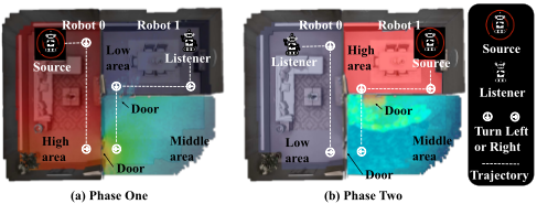
To overcome the aforementioned challenges, we propose MACMA (Measuring Acoustics with Collaborative Multiple Agents) which is illustrated in Figure 1). Both agents, one source (emitter) and one listener (receiver), learn a motion policy to perform significance sampling of RIR within any given 3D scene. The trained agents can move (according to the learned motion policy) in any new 3D scene to predict the RIR of that new scene. To achieve that, we design two policy learning modules: the RIR prediction module and the dynamic allocation module of environment reward. In Appx. B, we explore the design of environmental reward and based on this, and we further propose a reward distribution module to learn how to efficiently distribute the reward obtained at the current step, thereby incentivizing the two agents to learn to cooperate and move. To facilitate the convergence of optimization, we design loss functions separately for the policy learning module, the RIR prediction module, and the reward allocation module. Comparative experiments and ablation experiments are performed on two datasets Replica [Straub et al., 2019] and Matterport3D [Chang et al., 2017], verifying the effectiveness of the proposed solution. To the best of our knowledge, this work is the first RIR measurement method using two collaborative agents. The main contributions of this work are:
- we propose a new setting for planning RIR measuring under finite time steps and a solution to measure the RIR with two-agent cooperation in low resource situations;
- we design a novel reward function for the multi-agent decomposition to encourage coverage of environment acoustics;
- we design evaluation metrics for the collaborative measurement of RIR, and we experimentally verify the effectiveness of our model.
2 RelatedWork
RIR generation. Measuring the RIR has been of longstanding interest to researchers [Cao et al., 2016; Savioja and Svensson, 2015]. Traditional methods for generating RIR include statistical based methods [Schissler et al., 2014; Tang et al., 2022] and physics-based methods [Mehra et al., 2013; Taylor et al., 2012]. However, they are computationally prohibitive. Recent methods estimate the acoustics of RIR by parameters to generate RIR indirectly [Masztalski et al., 2020;
Diaz-Guerra et al., 2021; Ratnarajah et al., 2021]. Although these methods are flexible in extracting different acoustic cues, their predictions are independent of the source and receiver's exact locations, making them unsuitable for scenarios where the mapping between RIR and locations of source and receiver is important (e.g. sound source localization and audiovisual navigation). FAST-RIR [Ratnarajah et al., 2022b] is a GAN-based RIR generator that generates a large-scale RIR dataset capable of accurately modeling source and receiver locations, but for efficiency, they rely on handcrafted features instead of learning them, which affects generative fidelity [Luo et al., 2022]. Neural Acoustic Field (NAF) [Luo et al., 2022] addresses the issues of efficiency and fidelity by learning an implicit representation of RIR [Mildenhall et al., 2022], and by introducing global features and local embeddings. However, NAF cannot generalize to new environments, and its training time and model storage cost grows linearly with the number of environments [Majumder et al., 2022]. The recently proposed MESH2IR [Ratnarajah et al., 2022a] is an indoor 3D scene IR generator that takes the scene's mesh, listener positions, and source locations as input. MESH2IR [Ratnarajah et al., 2022a] and FAST-RIR [Ratnarajah et al., 2022b] assume that the environment and reverberation characteristics have been given, hence they only consider the fitting for the existing dataset, and ignore the measurement cost. However, our model considers how two moving agents collaborate to optimize RIR measuring from the aspects of time consumption, coverage, accuracy, etc. It is worth mentioning that our model addresses multiple scenarios, so that it is more suitable for generalizing to unseen environments.
Audio spatialization. Binaural audio generation methods comprise converting mono audio to binaural audio using visual information in video [Garg et al., 2021], utilizing spherical harmonics to generate binaural audio from mono audio for training [Xu et al., 2021], and generate binaural audio from video [Ruohan and Kristen, 2019]. Using 360 videos from YouTube to generate 360-degree ambisonic sound [Morgado et al., 2018] is a higher-dimensional audio spatialization. Alternatively, [Rachavarapu et al., 2021] directly synthesize spatial audio. Audio spatialization has a wide range of practical applications, such as object/speaker localization [Jiang et al., 2022], speech enhancement [Michelsanti et al., 2021], speech recognition [Shao et al., 2022], etc. Although all the above works use deep learning, our work is fundamentally different in that we propose to model binaural RIR measuring as a decision process (of two moving agents that learns to plan measurement) using time-series states as input.
Audio-visual learning. [Majumder et al., 2022] harnesses the synergy of egocentric visual and echogenic responses to infer ambient acoustics to predict RIR. The advancement of audiovisual learning has good applications in many tasks, such as audiovisual matching [Chen et al., 2022], audiovisual source separation [Majumder and Grauman, 2022] and audiovisual navigation [Chen et al., 2020; Dean et al., 2020; Gan et al., 2020; Gan et al., 2022; Yu et al., 2022a; Yu et al., 2023]. There are also work to use echo responses with vision to learn better spatial representations [Gao et al., 2020], infer depth [Christensen et al., 2020], or predict floor plans of 3D
environments [Purushwalkam et al., 2021]. The closest work to ours is audio-visual navigation, but audio-visual navigation has navigation goals, but the agents in our setup have no clear navigation destinations.
Multi-agent learning. There are two types of collaborative multi-agents: value decomposition based methods [Rashid et al., 2018; Rashid et al., 2020] and actor-critic [Foerster et al., 2018; Lowe et al., 2017] based methods. The centralized training with decentralized execution (CTDE) paradigm [Wang et al., 2021] has recently attracted attention for its ability to address non-stationarity while maintaining decentralized execution. Learning a centralized critic with decentralized actors (CCDA) is an efficient approach that exploits the CTDE paradigm. Multi-agent deep deterministic policy gradient (MADDPG) and counterfactual multi-agent (COMA) are two representative examples. In our design, we have a centralized critic (named Critic) with decentralized actors (named AgentActor0 and AgentActor1). But our task differs from all the above multi-agent learning methods in that the agents in our scenario are working on a collaborative task, while previous multi-agent learning research has mainly focused on competitive tasks.
3 The Proposed Approach
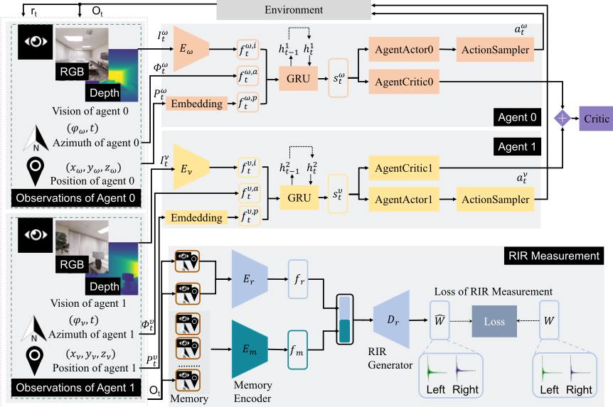
Our model MACMA has two collaborative agents moving in a 3D environment in Figure 1, using vision, position, and azimuth to measure the RIR. The proposed model mainly consists of three parts: agent 0, agent 1, and RIR measurement (see Figure 2). Given egocentric vision, azimuth, and position inputs, our model encodes these multi-modal cues to 1) determine the action for agents and evaluate the action taken by the agents for policy optimization, 2) measure the room impulse response and evaluate the regression accuracy for the RIR generator, and 3) evaluate the trade-off between the agents' exploration and RIR measurement. The two agents repeat this process until the maximal steps have been reached.
Specifically, at each step t (cf. Figure 2), the robots receive the current observation of their own Oω t and Oν t respectively, where Oω t = (I ω t , Φωt , P ω t ), Oν t = (I ν t , Φνt , P ν t ), I ω t = (I ω, rgb t , I ω, depth t ) and I ν t = (I ν, rgb t , I ν, depth t ) are egocentric visions for robot 0 and robot 1 respectively. Φωt = (φωt , t) and Φνt = (φν, t) are azimuths for robot 0 and robot 1 respectively. P ω t = (xω, yω, zω) and P ν t = (xv, yv, zv) are positions for robot 0 and robot 1 respectively. I ω t or I ν t denotes the current visual input that can be RGB (128×128×3 pixels) and/or depth (with a dimension of 128×128×1) image 1 , Φωt and Φνt are 2D vector with time. P ω t and P ν t are 3D vector. Although there exists a navigability graph (with nodes and edges) of the environment, this graph is hidden from the robot, hence the robots must learn from the accumulated observations Oω t and Oν t to understand the geometry of the scene. At each step, the robot at a certain node A can only move to another node B in the navigability graph if 1) an edge connects both nodes, and 2) the robot is facing node B. The viable robotic action space is defined as A ={MoveForward, TurnLeft, TurnRight, Stop}, where the Stop action should be executed when the robot completes the task or the number of the robot's actions reach the maximum number of steps. The overall goal is to predict RIR in new scene accurately and explore widely.
1 Both RGB and depth images capture the 90-degree field of view in front of the navigating robot.
3.1 ProblemFormulation
We denote agent 0 and agent 1 with superscript ω and ν, respectively. The game M = (S, (Aω ,Aν ),P, (Rω ,Rν )) consists of state set S, action sets (Aω , Aν ), a joint state transition function P : S ×Aω ×Aν → S, and the reward functions Rω : S × Aω × Aν × S → R for agent 0 and Rν : S×Aω ×Aν ×S → R for agent 1. Each player wishes to maximize their discounted sum of rewards. r is the reward given by the environment at every time step in an episode. MACMA is modeled as a multi-agent [Sunehag et al., 2018; Rashid et al., 2018] problem involving two collaborating players sharing the same goal:
where the loss L is defined in Equation 5. G(πω , πν , r) is the expected joint rewards for agent 0 and agent 1 as a whole. G(πω , r) and G(πν , r) are the discounted and cumulative rewards for agent 0 and agent 1, respectively. wω and wν denote the constant cumulative rewards balance factors for agent 0 and agent 1, respectively. ρω and ρν are immediate reward contributions for agent 0 and agent 1, respectively. ρ is a constant (throughout the training) reward allocation parameter. Inspired by Value Decomposition Networks (VDNs) [Sunehag et al., 2018] and QMIX [Rashid et al., 2018], we construct the objective function G(πω , πν , r) in Equation 1 by combining the non-negative partial reciprocal constraint respond to G(πω , r) and G(πν , r) (see theoretical details in Appx. A.1).
Agent 0, agent 1 and their optimization. The agent 0 and agent 1 receive the current observation Oω t = (I ω t , Φωt , P ω t ) and Oν t = (I ν t , Φνt , P ν t ) at the t-th step. The visual (I ω t and I ν t ) part is encoded into a visual feature vector using a CNN encoder: f ω, i t and f ν, i t (Eω for agent 0 and Eν for agent 1). Visual CNN encoders Eω and Eν are constructed in the same way (from the input to output layer): Conv8x8, Conv4x4, Conv3x3 and a 256-dim linear layer; ReLU activations are added between any two neighboring layers. P ω t and P ν t are embedded by an embedding layer and encoded into feature vectors f ω, p t and f ν, p t , respectively. Then, we concatenate the two vectors together with f ω, a t (Φωt ) and f ν, a t (Φνt ) to obtain the global observation embedding eωt = [f ω, i t , f ω, a t , f ω, p t ] and eνt = [f ν, i t , f ν, a t , f ν, p t ]. We transform the observation embeddings to state representations using a gated recurrent unit (GRU), sωt = GRU(eωt , h1t-1 ). We adopt a similar procedure to obtain sνt = GRU(eνt , h2t-1 ). The state vectors (sωt for agent 0 and sνt for agent 1) are then fed to an actor-critic network to 1) predict the conditioned action probability distribution πθω 1 (aωt |sωt ) for agent 0 and πθν 1 (aνt |sνt ) for agent 1, and 2) estimate the state value Vθω 2 (sωt , rω t ) for agent 0 and Vθω 2 (sνt , rν t ) for agent 1. The actor and critic are implemented with a single linear layer parameterized by θω 1 , θν 1 , θω 2 , and θν 2 , respectively. For the sake of conciseness, we use θ to denote the compound of θω 1 , θν 1 , θω 2 , and θν 2 hereafter. The action samplers in Figure 2 sample the actual action (i.e. aωt for agent 0 and aνt for agent 1) to execute from πθω 1 (aωt |sωt ) for agent 0 and πθν 1 (aνt |sνt ) for agent 1, respectively. Both agent 0 and agent 1 optimize their policy by maximizing the expected cumulative rewards G(πω , r) and G(πν , r) respectively in a discounted form. The Critic module evaluates the actions taken by agent 0 and agent 1 to guide them to take an improved action at the next time step. The loss of Lm is formulated as Equation 2.
where Lωm and Lνm are motion loss for agent 0 and agent 1 respectively, wωm,wνm are hyperparameters. The loss Ljm is defined as
where j ∈ {ω, ν}, and the estimated state value of the target network for j is denoted as ˆ Vθj (s). Vj (s) = maxa∈Aj E[rt + γ · Vj (st+1) | st = s]. The advantage for a given length-T trajectory is: ˆAjt = ∑T-1 i=t γ i+2-t · δj i , where δj t = rt + γ · Vj (st+1) - Vj (st). H(πθj (a | s)) is entropy of πθj (a | s). We collectively denote all the weights in Figure 2 except the above actor-critic network for agent 0 and agent 1 as Ω hereafter for simplicity.
RIR measurement and its regression. We encode the observations Oω t and Oν t with encoder Er, and the output of the encoder Er is fr. The historical observations Oω t+1-κ , Oν t+1-κ , · · · , Oω t-1 , Oν t-1 , Oω t , Oν t are sorted in the memory, and are encoded by Em outputting fm, where κ is the length of the memory bank. Then, fr and fm are concatenated. The predicted RIR ˆWt is obtained using RIR generator Dr. For more details on the structure of Er, Em and Dr, please refer to Appx. A.2. RIR measurement is learned with the ground truth RIR Wt. Lξ denote the loss of RIR measurement. Lξ are formulated as
where ˆWt is the predicted RIR from the RIR Measurement module. Wt is the ground truth RIR. ∆(Wt, ˆWt) is STFT (Short-time Fourier transform) distance. It is calculated by Equation 8. 10 and 4464.2 are experimental parameters from grid search.
The total evaluation. The Critic module is implemented with a linear layer. The total loss of our model is formulated as Equation 5. We minimize L following Proximal Policy Optimization (PPO) [Schulman et al., 2017].
where Lm is the loss component of motion for two agents, Lξ is the loss component of room impulse response prediction, wm and wξ are hyperparameters. The losses Lm and Lξ are formulated in Equation 2 and Equation 4, respectively.
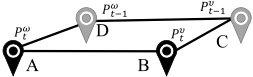
The design of environmental reward. It can be seen from Figure 3 that the ΓABCD is formed by the positions of the two agents at the current time step and the previous time step. rt is the current step reward, which is calculated by the following Equation 6.
ξ denotes the prediction of room impulse response. ζ denotes coverage rate. ψ denotes the length of the perimeter of the convex hull. ϕ denotes the area of the perimeter of the convex hull.
Among them, rξ t is the reward component in terms of measurement accuracy, which evaluates the improvement of the reward of the measurement accuracy of the current step and the reward of the measurement accuracy of the previous step. rξ t is calculated by
where ξt is the measurement accuracy of the current step. As briefly explained before, ∆(Wt, ˆWt) is the STFT distance that can be calculated by
where z is the magnitude spectrogram of ground truth RIR Wt for the current time step, while ˆ z is the corresponding predicted variant. Θ(z, ˆ z) is the average loss of spectral convergence for z and ˆ z; and Ξ(z, ˆ z) is the log STFT magnitude loss. Θ(z, ˆ z) and Ξ(z, ˆ z) are computed with
where ∥·∥F is Frobenius Norm. z = Λ(Wt) = √y2 r + y2 i , where yr is real part of STFT transform 2 of Wt, yi is an imaginary part of the result of the STFT transform of Wt. ˆ z = Λ( ˆWt) is defined similarly to z, and the calculation process of both z and ˆ z are the same.
2 The parameters for STFT transform are #FFT=1024, #shift =120, #window=600, window="Hamming window".
Algorithm 1 MACMA (Measuring Acoustics with Collaborative Multiple Agents)
Input: Environment E, # updates M, # episode N, max time steps T .
Parameter: Stochastic policies π, initial actor-critic weights θ0, initial other weights except for actor-critic weights Ω0. Output:Trained weights, θM and ΩM.
- 1: for i=1, 2, ... M do
- 2: // Run policy πθi-1 for N episodes T time steps
- 3: {(ot,i, ht-1,i, at,i, rt,i)} ← roll(E, πθi-1 , T)
- 4: Compute advantage estimates
- 5: RIR prediction and environmental reward assignment
- 6: // Optimize w.r.t. θ and Ω
- 7: θi,Ωi ←newθ andΩfromPPOalgorithmw.r.t. minimizing Equation 5
- 8: end for
ζt is the coverage of the current step, which is the ratio of visited nodes (only one duplicate node is counted) to all nodes in the scene at time step t. We calculate rζ t by
ψt and ϕt are respectively the perimeter and area of ΓABCD in Figure 3 at time step t. We calculate rψ t and rϕ t with
Overall algorithm. The entire procedure of MACMA is presented as pseudo-code in Algorithm 1.
4 Experiments
We adopt the commonly used 3D environments collected using the SoundSpaces platform [Chen et al., 2020] and Habitat simulator [Savva et al., 2019]. They are publicly available as several datasets: Replica [Straub et al., 2019], Matterport3D [Chang et al., 2017] and SoundSpaces (audio) [Chen et al., 2020]. Replica contains 18 environments in the form of grids (with a resolution of 0.5 meters) constructed from accurate scans of apartments, offices, and hotels. Matterport3D has 85 scanned grids (1-meter resolution) of indoor environments like personal homes. To measure the RIR in Replica [Straub et al., 2019] and Matterport3D [Chang et al., 2017], we let two agents move a certain number of steps (250 and 300 steps for Replica and Matterport3D, respectively) throughout the scene and plan a measuring path. At every time step, the two agents measure the RIR while moving. The experimental procedure contains several phases: a) we pretrain generator Dr under the setting L = Lm (wm = 1.0 and wξ = 0.0) with random policy for both agent 0 and agent 1 in the training split, b) we train and validate every baseline with the generator Dr fine-tune together in the training and validation split, c) we test every baseline in the test split. MACMA is benchmarked towards several baselines: Random, Nearest neighbor, Occupancy [Ramakrishnan et al., 2020] and Curiosity [Pathak et al., 2017]. Random uniformly samples one of three actions and executes Stop when it reaches maximum steps. Nearest neighbor predict from closest experience (Appx. A.3). Occupancy orient to occupy more area, making the area of ΓABCD in Figure 3 larger. Curiosity strives to visit nodes that have not been visited already in the current episode. To evaluate different methods, we adopt the evaluation metrics CR (coverage rate), PE (prediction error),WCR (weighted coverage rate),RTE (RT60 Error) and SiSDR (scale-invariant signalto-distortion ratio), among which WCR is the most important evaluation metric since it is a trade-off between encouraging high prediction accuracy and more exploration. CR is the ratio of the number of visited nodes by agents and the number of nodes in the current episode. CR = Nv/Ne, where Nv is the total number of unique nodes that two agents have visited together, and Ne is the total number of all individual nodes in the current episode. PE = ∆(Wt, ˆWt), where Wt (Equation 8) is the ground truth RIR, ˆWt is the predicted RIR. WCR = (1.0 - λ) ∗ CR + λ ∗ (1.0 - PES), where PES stands for Scaled Prediction Error. PES = 2/(1+exp(-PE))-1.0, where 0 ≤ λ ≤ 1.0 is a hyper-parameter. RTE describes the difference between the ground truth RT60 value and the predicted one. SiSDR = 10 log10 ∥XT ∥2/∥XE∥2 , where ∥XE∥2 is the error vector and ∥XT∥2 is the ground truth vector. We select the hyperparameters in grid search and the details are in Appx. A.4.
4.1 Experimental Results
Results are averages of 5 tests with different random seeds. Quantitative comparison of the two datasets. Results are runs on two datasets under the experimental settings: αξ =1.0, αζ =1.0, αψ =-1.0, αϕ=1.0, κ=2, λ=0.1, ρ=-1.0. As seen from Table 1, on the Replica dataset, MACMA achieves the best results on the metrics WCR, PE and CR. But the Curiosity model has the best results on the metrics RTE and SiSDR. The Curiosity model encourages agents to visit more new nodes near them, which drive up the robots' exploration ability (it improves performance on metrics RTE and SiSDR) while reducing their team's performance (it reduces performance on the metric CR). The Occupancy model (ranks as the second over CR) motivates the exploratory ability of the entire group (the group of agent 0 and agent 1) but ignores their individual exploration performance (the ranks over the metrics of RTE and SiSDR lower than that of CR). MACMA combines the group exploration ability and the individual exploration ability, achieving a good trade-off between the two abilities, so that the group exploration ability of MACMA has increased by a large margin (e.g. over the CR metric) and finally won the championship on the WCR metric. On the Matterport3D dataset, MACMA achieves the best results on all metrics. As a result, we can conclude that MACMA quantitatively outperforms baselines over both datasets.
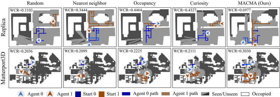
Qualitative comparison on exploration capability. Figure 4 shows the navigation trajectories of agent 0 and agent 1 for different algorithms by the end of a particular episode from the Replica (top row) and Matterport3D (bottom row) dataset. The light-gray areas in Figure 4 indicate the exploration field of the robots. We observe that MACMA tends to explore the most extensively compared to the other baselines. Particularly, there are three rooms in the entire scene in Replica, and MACMA is the only method that managed to traverse all three rooms using the same number of time steps as baselines.
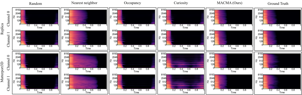
Qualitative comparison on RIR prediction. We show the spectrograms generated by these models and from the ground truth in Figure 5. These binaural spectrograms with channel 0 and channel 1 last for one second (the x-axis is the time axis). The spectrogram of the RIR from both Random's and Occupancy's generation have fewer color blocks than the ground truth between 0.2 seconds and 0.4 seconds and more color blocks than the ground truth between 0.8 seconds and 1 second. The spectrogram of the RIR from the Nearest neighbor's generation has more colored regions than the ground truth spectrogram. The spectrogram of the RIR from Curiosity's prediction has fewer color blocks than the ground truth between 0.2 seconds and 0.4 seconds. At the same time, the spectrogram of the RIR from Curiosity's generation has more color blocks than the ground truth between 0.8 seconds and 1 second in the Replica dataset. And the spectrogram of the RIR from Curiosity's prediction has more colored regions than the ground truth spectrogram in the Matterport3D dataset. The spectrogram of the generated RIR from MACMA (Ours) is the closest to the ground truth spectrogram. In conclusion, from a qualitative human visual point of view, the spectral quality of the RIRs generated by our model is the best. Additionally, in Appx. A.5, we show that the RIR's quality in the waveform of the RIRs generated by our model is also superior.
4.2 Ablation Studies
Ablation on modality. Results are run on dataset Replica under the experimental settings of αξ =1.0, αζ =1.0, αψ =-1.0, αϕ=1.0, κ=2, λ=0.1, ρ=-1.0. As shown in Table 2, RGBD (vision with RGB images and Depth input) seems to be the best choice.
More ablations. We explore the relationship between modality importance, action selection, and RIR measurement accuracy in Appx. A.6 and Appx. A.7. We present the extension model MACMARA (MACMA with a dynamic Reward Assignment module) in Appx. B.5. More ablation studies on memory size κ and the reward component can be found in Appx. A.4.
5 Conclusion
In this work, we propose a novel task where two collaborative agents learn to measure room impulse responses of an environment by moving and emitting/receiving signals in the environment within a given time budget. To tackle this task, we design a collaborative navigation and exploration policy. Our approach outperforms several other baselines on the environment's coverage and prediction error. A known limitation is that we only explored the most basic setting, one listener (receiver), and one source (emitter), and did not study the settings with two or more listeners or sources. Another limitation of our work is that our current assessments are conducted in a virtual environment. It would be more meaningful to evaluate our method on real-world cases, such as a robot moving in a real house and learning to measure environmental acoustics collaboratively. Lastly, we have not considered semantic information about the scene in policy learning. Incorporating semantic information about the scene into policy learning would be more meaningful. The above three are left for future exploration.
| Model | Replica | Matterport3D | ||||||||
|---|---|---|---|---|---|---|---|---|---|---|
| WCR (↑) | PE (↓) | CR (↑) | RTE (↓) | SiSDR (↑) | WCR (↑) | PE (↓) | CR (↑) | RTE (↓) | SiSDR (↑) | |
| Random | 0.3103 | 5.4925 | 0.3439 | 14.7427 | 20.3534 | 0.2036 | 5.5552 | 0.2254 | 23.5281 | 12.3042 |
| Nearest neighbor | 0.3444 | 5.4533 | 0.3817 | 14.0269 | 22.0135 | 0.2099 | 5.3342 | 0.2321 | 28.8765 | 15.2351 |
| Occupancy | 0.4464 | 3.7224 | 0.4907 | 12.5532 | 23.0666 | 0.2225 | 4.5327 | 0.2449 | 20.3399 | 18.3848 |
| Curiosity | 0.4327 | 3.4883 | 0.4742 | 10.9565 | 23.8669 | 0.2111 | 4.4255 | 0.2319 | 29.5572 | 20.0031 |
| MACMA (Ours) | 0.6977 | 3.2509 | 0.7669 | 13.8896 | 23.6501 | 0.3030 | 4.0113 | 0.3327 | 15.9338 | 21.3187 |
| Vision | WCR (↑) | PE (↓) | CR (↑) | RTE (↓) | SiSDR (↑) |
| Blind | 0.5020 | 3.4966 | 0.5512 | 14.2049 | 23.0903 |
| RGB | 0.5930 | 3.8204 | 0.6541 | 15.5897 | 23.7713 |
| Depth | 0.5068 | 3.4927 | 0.5566 | 29.6905 | 23.5089 |
| RGBD | 0.6977 | 3.2509 | 0.7669 | 13.8896 | 23.6501 |
Ethical Statement
This research follows IJCAI's ethics guidelines and does not involve human subjects or privacy issues with the dataset. The dataset is publicly available.
Acknowledgments
We thank the IJCAI 2023 reviewers for their insightful feedback. This work is supported by multiple projects, including the Sino-German Collaborative Research Project Crossmodal Learning (NSFC62061136001/DFG SFB/TRR169), the National Natural Science Foundation of China (No. 61961039), the National Key R&D Program of China (No. 2022ZD0115803), the Xinjiang Natural Science Foundation
(No. 2022D01C432, No. 2022D01C58, No. 2020D01C026, and No. 2015211C288), and partial funding from the THUBosch JCML Center.
@inproceedings{ijcai2023p38,
  title     = {Measuring Acoustics with Collaborative Multiple Agents},
  author    = {Yu, Yinfeng and Chen, Changan and Cao, Lele and Yang, Fangkai and Sun, Fuchun},
  booktitle = {Proceedings of the Thirty-Second International Joint Conference on
               Artificial Intelligence, {IJCAI-23}},
  publisher = {International Joint Conferences on Artificial Intelligence Organization},
  editor    = {Edith Elkind},
  pages     = {335--343},
  year      = {2023},
  month     = {8},
  note      = {Main Track},
  doi       = {10.24963/ijcai.2023/38},
  url       = {https://doi.org/10.24963/ijcai.2023/38},
}
TY - CPAPER TI - Measuring Acoustics with Collaborative Multiple Agents AU - Yu, Yinfeng AU - Chen, Changan AU - Cao, Lele AU - Yang, Fangkai AU - Sun, Fuchun T2 - Proceedings of the Thirty-Second International Joint Conference on Artificial Intelligence, IJCAI-23 PB - International Joint Conferences on Artificial Intelligence Organization PY - 2023 SP - 335 EP - 343 DO - 10.24963/ijcai.2023/38 UR - https://doi.org/10.24963/ijcai.2023/38 ER -Copied
Machine-readable versions of this paper, for tools and AI agents:





