
Autonomous Exploration for Navigating in MDPs Using Blackbox RL Algorithms
Proceedings of the Thirty-Second International Joint Conference on Artificial Intelligence. Main Track. Pages 3714-3722.
https://doi.org/10.24963/ijcai.2023/413
Keywords
- Machine Learning: ML: Reinforcement learning
- Machine Learning: ML: Learning theory
Abstract
We consider the problem of navigating in a Markov decision process where extrinsic rewards are either absent or ignored. In this setting, the objective is to learn policies to reach all the states that are reachable within a given number of steps (in expectation) from a starting state. We introduce a novel meta-algorithm which can use any online reinforcement learning algorithm (with appropriate regret guarantees) as a black-box. Our algorithm demonstrates a method for transforming the output of online algorithms to a batch setting. We prove an upper bound on the sample complexity of our algorithm in terms of the regret bound of the used black-box RL algorithm. Furthermore, we provide experimental results to validate the effectiveness of our algorithm and correctness of our theoretical results.
- [Achiam and Sastry, 2017] Joshua Achiam and Shankar Sas- try. Surprise-based intrinsic motivation for deep reinforce- ment learning. CoRR, abs/1703.01732, 2017.
- [Agarwal et al., 2020] Alekh Agarwal, Mikael Henaff, Sham Kakade, and Wen Sun. Pc-pg: Policy cover directed explo- ration for provable policy gradient learning. In Advances in Neural Information Processing Systems, volume 33, 2020.
- [Azar et al., 2019] Mohammad Gheshlaghi Azar, Bilal Piot, Bernardo A. Pires, Jean-Bastien Grill, Florent Altché, and Rémi Munos. World discovery models. CoRR, abs/1902.07685, 2019.
- [Azuma, 1967] Kazuoki Azuma. Weighted sums of cer- tain dependent random variables. Tohoku Math. J. (2), 19(3):357-367, 1967.
- [Baranes and Oudeyer, 2009] A. Baranes and P.-Y. Oudeyer. R-IAC: Robust intrinsically motivated exploration and ac- tive learning. IEEE Transactions on Autonomous Mental Development, 1:155-169, 2009.
- [Bartlett and Tewari, 2009] Peter L. Bartlett and Ambuj Tewari. Regal: A regularization based algorithm for reinforcement learning in weakly communicating mdps. In Proceedings of the Twenty-Fifth Conference on Un- certainty in Artificial Intelligence, UAI '09, page 35-42, 2009.
- [Burda et al., 2019] Yuri Burda, Harrison Edwards, Deepak Pathak, Amos J. Storkey, Trevor Darrell, and Alexei A. Efros. Large-scale study of curiosity-driven learning. In ICLR, 2019.
- [Cai et al., 2022] Haoyuan Cai, Tengyu Ma, and Simon Du. Near-optimal algorithms for autonomous exploration and multi-goal stochastic shortest path. In Kamalika Chaud- huri, Stefanie Jegelka, Le Song, Csaba Szepesvari, Gang Niu, and Sivan Sabato, editors, Proceedings of the 39th International Conference on Machine Learning, volume 162 of Proceedings of Machine Learning Research, pages 2434-2456. PMLR, 17-23 Jul 2022.
- [Cesa-Bianchi et al., 1997] Nicolò Cesa-Bianchi, Yoav Fre- und, David Haussler, David P. Helmbold, Robert E. Schapire, and Manfred K. Warmuth. How to use expert advice. J. ACM, page 427-485, May 1997.
- [Cesa-Bianchi et al., 2006] Nicolò Cesa-Bianchi, Alex Con- coni, and Claudio Gentile. On the generalization ability of on-line learning algorithms. IEEE Trans. Inf. Theor., 50(9):2050-2057, September 2006.
- [Ecoffet et al., 2019] Adrien Ecoffet, Joost Huizinga, Joel Lehman, Kenneth O. Stanley, and Jeff Clune. Go-explore: a new approach for hard-exploration problems. CoRR, abs/1901.10995, 2019.
- [Ecoffet et al., 2020] Adrien Ecoffet, Joost Huizinga, Joel Lehman, Kenneth O. Stanley, and Jeff Clune. First return then explore. CoRR, abs/2004.12919, 2020.
- [Florensa et al., 2018] Carlos Florensa, David Held, Xinyang Geng, and Pieter Abbeel. Automatic goal gener- ation for reinforcement learning agents. In Proceedings of the 35th International Conference on Machine Learning, volume 80 of Proceedings of Machine Learning Research, pages 1515-1528. PMLR, 10-15 Jul 2018.
- [Freund and Schapire, 1999] Yoav Freund and Robert E. Schapire. Large margin classification using the perceptron algorithm. Mach. Learn., page 277-296, 1999.
- [Fruit et al., 2020] Ronan Fruit, Matteo Pirotta, and Alessan- dro Lazaric. Improved analysis of UCRL2 with empirical bernstein inequality. CoRR, abs/2007.05456, 2020.
- [Gajane et al., 2019] Pratik Gajane, Ronald Ortner, Peter Auer, and Csaba Szepesvári. Autonomous explo- ration for navigating in non-stationary cmps. CoRR, abs/1910.08446, 2019.
- [Gottlieb et al., 2013] Jacqueline Gottlieb, Pierre-Yves Oudeyer, Manuel Lopes, and Adrien Baranes. Information-seeking, curiosity, and attention: com- putational and neural mechanisms. Trends in cognitive sciences, 17(11):585-593, 2013.
- [Haber et al., 2018] Nick Haber, Damian Mrowca, Stephanie Wang, Li F Fei-Fei, and Daniel L Yamins. Learning to play with intrinsically-motivated, self-aware agents. In Advances in Neural Information Processing Systems, pages 8388-8399, 2018.
- [Hazan et al., 2019] Elad Hazan, Sham Kakade, Karan Singh, and Abby Van Soest. Provably efficient maximum entropy exploration. In Kamalika Chaudhuri and Ruslan Salakhutdinov, editors, ICML, volume 97, pages 2681- 2691, 2019.
- [Helmbold and Warmuth, 1995] David P. Helmbold and Manfred K. Warmuth. On weak learning. J. Comput. Syst. Sci., page 551-573, June 1995.
- [Hoeffding, 1963] Wassily Hoeffding. Probability inequali- ties for sums of bounded random variables. Journal of the American Statistical Association, 58(301):13-30, 1963.
- [Houthooft et al., 2016] Rein Houthooft, Xi Chen, Yan Duan, John Schulman, Filip De Turck, and Pieter Abbeel. Variational information maximizing exploration. In NIPS 2016 Deep Learning Symposium, 2016.
- [Jaksch et al., 2010] Thomas Jaksch, Ronald Ortner, and Pe- ter Auer. Near-optimal regret bounds for reinforce- ment learning. Journal of Machine Learning Research, 11(51):1563-1600, 2010.
- [Jin et al., 2020] Chi Jin, Akshay Krishnamurthy, Max Sim- chowitz, and Tiancheng Yu. Reward-free exploration for reinforcement learning. In Proceedings of the 37th Inter- national Conference on Machine Learning, volume 119 of Proceedings of Machine Learning Research, pages 4870- 4879. PMLR, 2020.
- [Kaplan and Oudeyer, 2003] Frédéric Kaplan and Pierre- Yves Oudeyer. Motivational principles for visual know- how development. Lund University Cognitive Studies, 101:73-80, 2003.
- [Lim and Auer, 2012] Shiau Hong Lim and Peter Auer. Au- tonomous exploration for navigating in mdps. In Proceed- ings of the 25th Annual Conference on Learning Theory, volume 23 of Proceedings of Machine Learning Research, pages 40.1-40.24, 2012.
- [Littlestone, 1989] Nick Littlestone. From on-line to batch learning. In Proceedings of the Second Annual Work- shop on Computational Learning Theory, COLT '89, page 269-284, 1989.
- [Lopes et al., 2012] Manuel Lopes, Tobias Lang, Marc Tou- ssaint, and Pierre-Yves Oudeyer. Exploration in model- based reinforcement learning by empirically estimating learning progress. In Advances in neural information pro- cessing systems, pages 206-214, 2012.
- [Ostrovski et al., 2017] Georg Ostrovski, Marc G Bellemare, Aäron van den Oord, and Rémi Munos. Count-based ex- ploration with neural density models. In Proceedings of the 34th International Conference on Machine Learning, pages 2721-2730, 2017.
- [Oudeyer and Kaplan, 2007] Pierre-Yves Oudeyer and Frédéric Kaplan. What is intrinsic motivation? a typology of computational approaches. Frontiers in neurorobotics, 1, 2007.
- [Pathak et al., 2017] Deepak Pathak, Pulkit Agrawal, Alexei A Efros, and Trevor Darrell. Curiosity-driven exploration by self-supervised prediction. In Proceedings of the IEEE Conference on Computer Vision and Pattern Recognition Workshops, pages 16-17, 2017.
- [Schmidhuber, 2010] Jürgen Schmidhuber. Formal theory of creativity, fun, and intrinsic motivation (1990-2010). Autonomous Mental Development, IEEE Transactions on, 2:230-247, 2010.
- [Shalev-Shwartz, 2012] Shai Shalev-Shwartz. Online learn- ing and online convex optimization. Found. Trends Mach. Learn., 4(2):107-194, February 2012.
- [Singh et al., 2004] Satinder P. Singh, Andrew G. Barto, and Nuttapong Chentanez. Intrinsically motivated reinforce- ment learning. In NIPS, 2004.
- [Singh et al., 2010] Satinder P. Singh, Richard L. Lewis, An- drew G. Barto, and Jonathan Sorg. Intrinsically moti- vated reinforcement learning: An evolutionary perspec- tive. IEEE T. Autonomous Mental Development, 2:70-82, 2010.
- [Tarbouriech et al., 2019] Jean Tarbouriech, Evrard Garcelon, Michal Valko, Matteo Pirotta, and Alessan- dro Lazaric. No-regret exploration in goal-oriented reinforcement learning. CoRR, abs/1912.03517, 2019.
- [Tarbouriech et al., 2020] Jean Tarbouriech, Matteo Pirotta, Michal Valko, and Alessandro Lazaric. Improved sam- ple complexity for incremental autonomous exploration in mdps. In Advances in Neural Information Processing Sys- tems 33 pre-proceedings (NeurIPS 2020), 2020.
- [Weng et al., 2001] Juyang Weng, James McClelland, Alex Pentland, Olaf Sporns, Ida Stockman, Mriganka Sur, and Esther Thelen. Autonomous mental development by robots and animals. Science, 291(5504):599-600, 2001.
References were extracted automatically from the PDF and may contain errors.
Full text extracted automatically from the PDF; figures, tables and equations may differ. The PDF is the version of record.
1 Introduction
The ability to efficiently explore the environment remains key to sample-efficient reinforcement learning (RL). In settings where rewards are absent or sparse, the exploration must be autonomous, i.e., it cannot be guided by reward maximization. Furthermore, many works have argued for a learning approach in which the agent undergoes an extended developmental period during which reusable skills are autonomously learned that will be useful for a wide range of challenges later (e.g., [Kaplan and Oudeyer, 2003; Weng et al., 2001]). In this article, we focus on learning to navigate in an unknown environment using such an approach.
Following [Lim and Auer, 2012], we consider a Markov decision process (MDP) equipped with at most countably many states and finitely many actions including a reset action which brings the agent back to some initial state. No extrinsic rewards are given and the state-transition probabilities are assumed to be stationary. The goal is to minimize the number of steps required by the agent to learn to reliably navigate to all reachable states. Since the number of states is unbounded, the agent is given as input a "radius" L such that it needs to consider all the states that are reachable within L steps (precise definitions will follow in the next section). This framework is particularly suitable when the task is to explore a large-scale environment and the learner only has enough resources to observe a small part of it by autonomous exploration. In such scenarios, it is imperative that the learner first solves simpler intrinsic goal-oriented tasks prescribed by the given number of steps L. This model could also be used in scenarios where the goal is to learn the transition operator directly.
1.1 RelatedWork
Similar problems have been considered in various research communities under the name of learning using intrinsic motivation/reward, curiosity-driven learning, automatic goal generation etc. Owing to the space restrictions, a necessarily incomplete list of these works include [Schmidhuber, 2010; Singh et al., 2004; Singh et al., 2010; Oudeyer and Kaplan, 2007; Baranes and Oudeyer, 2009; Lopes et al., 2012; Gottlieb et al., 2013; Houthooft et al., 2016; Achiam and Sastry, 2017; Ostrovski et al., 2017; Pathak et al., 2017; Haber et al., 2018; Burda et al., 2019; Azar et al., 2019; Hazan et al., 2019; Florensa et al., 2018]. Recently, [Ecoffet et al., 2019; Ecoffet et al., 2020] have proposed a family of algorithms for exploration when rewards are sparse or deceptive with experimental validation for the performance of their algorithms. Our approach could be applicable in scenarios similar to the ones considered in [Ecoffet et al., 2019; Ecoffet et al., 2020] who also exploit the same principle employed in our article - remember promising states and first return to such states before intentionally exploring.
[Gajane et al., 2019] consider a variant of the problem at hand where the transition probabilities can change abruptly. Another line of work is presented by [Tarbouriech et al., 2020] in which the authors consider a slightly modified goal (see [Tarbouriech et al., 2020, Definition 5] for more details). Recently, [Cai et al., 2022] proved a lower bound, based on the lower bound of UCRL2 [Jaksch et al., 2010], for the considered problem. Another relevant work is the "reward-free RL" paradigm introduced by [Jin et al., 2020]: following its exploration phase, their algorithm is able to compute nearoptimal policies for a collection of given reward functions. Although related to the problem at hand at a conceptual level, their approach remains limited to the finite-horizon setting. While we focus on showing how a general RL algorithm can be used for the task of exploration, another line of work (e.g., [Agarwal et al., 2020]) studies how exploration algorithms (i.e., policy cover) can be turned into a general RL algorithm.
Our proposed algorithm shares some ideas with "online-tobatch" conversion methods [Littlestone, 1989; Cesa-Bianchi et al., 2006]. It has been showed that one can obtain expected risk bounds for a hypothesis drawn randomly among those generated from online learning algorithms [Helmbold and Warmuth, 1995; Freund and Schapire, 1999; Cesa-Bianchi et al., 1997]. [Shalev-Shwartz, 2012] prove that if we have an online learning algorithm that is guaranteed to have low regret, then the cost of such a random hypothesis is close to the optimal cost.
1.2 Main Contribution
We show that any RL algorithm with sublinear regret T α, α < 1, can be converted into an exploration algorithm. To the best of our knowledge, our work provides the inaugural algorithm to convert any RL algorithm with sublinear regret into an exploration algorithm with suitable guarantees on its sample complexity. This formally verifies the intuition that any small regret algorithm needs to explore its environment, at least implicitly. This also shows that RL algorithms that take advantage of a particular transition structure of an environment, resulting in improved regret bounds, can be converted into a corresponding exploration algorithm for this environment. Our black-box approach of using an RL algorithm as a subroutine leads to the generality of our proposed solution, which is one its main strengths. The structure of the proposed algorithm and its analysis may also serve as a worthy addition to the literature of online-to-batch conversion methods.
2 Problem Setting
In this section, we present the problem setting first introduced by [Lim and Auer, 2012] 1 . We consider a discrete-time Markov decision process M with no external rewards. We assume a countable, possibly infinite state space S and a finite action space A. Upon executing an action a in state s, the environment moves to the next state s′ selected randomly according to the unknown transition probabilities P(s′ |s, a).
The learning agent is expected to solve the autonomous exploration problem in which the goal is to find a policy for each state reachable from a starting state. In the following, we assume (without loss of generality) the starting state s0 to be fixed, and hence it will be omitted from any notation.
Definition 1 (Navigation time). For any policy π, let τπ(s) be the expected number of steps before reaching s for the first time when executing policy π starting from s0.
We further set τ ∗ (s) :=minπ τπ(s). The learner will be given a number L > 0 and we may naively demand that it finds all the states reachable in at most L steps:
Definition 2 (L-reachable states). We let SL denote the set of all the states reachable in at most L steps i.e.,
Since the state space might be infinite, a learner could wander off in some direction or get stuck without being able to return to the starting state. To exclude this possibility, we make Assumption 1.
1 Readers may consult the list of symbols given in the extended version of this article to quickly look up the notation.
Assumption 1. In every state s, there is a designated RESET action available, such that P (s0|s, RESET) = 1.
Definition 3 (Policy on S′ ⊂ S). We define a policy π on S′ ⊂ S to be a policy with π(s) = RESET for any s ̸∈ S′ .
[Lim and Auer, 2012] show that, in general, efficient learning to discover all the states in SL is not possible. Rather, we require the learners to discover only the incrementally reachable states, S→L .
Definition 4 (Incrementally reachable states). Let ≺ be some partial order on S. The set S≺L of states reachable in L steps with respect to ≺, is defined inductively as follows:
- s0 ∈ S≺L ,
- if there is a policy π on {s′ ∈ S≺L : s′ ≺ s} with τπ(s) ≤ L, then s ∈ S≺L .
We define the set S→L of states incrementally reachable in L steps with respect to some partial order to be S→L := ⋃≺ S≺L , where the union is over all possible partial orders.
As [Lim and Auer, 2012], we are interested in the number of exploration steps needed to be able to navigate to incrementally reachable states from s0 efficiently. Thus, given parameters L and ϵ, a suitable exploration algorithm will be able to determine
- a set K⊇ S→L , and
- for every s ∈ K, a policy πs with τπs (s) ≤ (1+ ϵ)L,
after a certain number of exploration steps dependent on L and ϵ.
3 Algorithm andMain Result
In this section, we present our proposed algorithm called META-EXPLORE (given in Algorithm 1) and an upper bound on its number of exploration steps. The motivation for using a black-box approach in META-EXPLORE is that it provides the generality of converting an arbitrary online RL algorithm into an exploration algorithm. The main idea of META-EXPLORE is to consider reaching a particular state as a sub-problem that is solved by using an arbitrary online RL algorithm A with regret guarantees (e.g. UCRL2 from [Jaksch et al., 2010], REGAL from [Bartlett and Tewari, 2009]). To reach a particular state, several hypotheses (defined in Section 3.1 below) are formed using the black-box RL algorithm A.
META-EXPLORE proceeds in rounds. In each round, it evaluates a target state to examine if a (1 + ϵ)L-step policy for that state can be found, for a given threshold ϵ. At the end of a particular round, if the algorithm determines (with high confidence) that a (1 + ϵ)L-step policy for the chosen target state has been found, the round is deemed a success round, otherwise it is called a failure round. At the end of a successful round, the chosen target state is added to the set of "known" states K. On the other hand, at the end of a failure round, the algorithm is said to have rejected the target state. The algorithmmaintains another set U, called the set of candidate states i.e., states that are potential members of S→L . Note that, in any round, the algorithm tries to find a policy on K at that time in order to reach the target state.
3.1 Major Steps of the Algorithm
Each round consists of three steps - state discovery, choice of target state, and target state evaluation.
State Discovery
Whenever the algorithm discovers a new known state snew, it explores the neighborhood of snew to add to the set of candidate states U. That is, in snew every action a ∈ A is sampled ⌈L log 8AL|K|2 δ ⌉ times. By definition of a known state, the algorithm has a (1+ϵ)L-step policy πsnew to reach snew from the starting state s0. To sample any action a ∈ A in snew, the algorithm first resets to s0 and then uses πsnew to reach snew. Thus, sampling each action once requires on average (1 + ϵ)L + 1 steps at most. Any neighboring states of snew which are not already in K are added to U. The algorithm also keeps hold of the neighboring states discovered by each known state. Every time a new state becomes known, all the neighboring states {s} of the previously known states such that s /∈ K are also added to the set of candidate states U. Note that a neighboring state is added to U even if it has been previously rejected by the algorithm. This is done to ensure that if a target state sr ∈ S→L is erroneously rejected by the algorithm because the preceding states from some partial order (see Definition 4) were not in K at that time, sr will be considered as a target state again (this reasoning is explained in detail in Section 4.5 below).
Choice of Target State
The target state for the current round is chosen arbitrarily without replacement from the set of candidate states U. The algorithm stops when U is empty.
Target State Evaluation
This step forms the crux of the algorithm. Consider a round r with target state ¯ s. Let us define an environmental episode (or, simply an episode) as a series of time steps beginning at the initial state s0 and ending when ¯ s is reached. An online RL algorithm A (with given regret guarantees) is run on the induced MDP M¯ s for Λ environmental episodes, where Λ is as defined in Step 3 in Algorithm 1.
Definition 5 (Induced MDP). In the induced MDP M¯ s, all the actions in state ¯ s suffer loss 0 and lead back to the initial state. All the states {s|s /∈ K∧ s ̸= ¯ s} are merged into a single auxiliary state at which only the RESET action is possible suffering loss 1. Actions in all the other states behave the same as in the original MDP and suffer loss 1.
Thus, minimizing the total loss inM¯ s is equivalent to minimizing the number of steps to reach the target state ¯ s.
At the beginning of each episode, the history of A in the current round is recorded. The recorded history comprises the state-action-state transition counts from the current round.
Definition 6 (Hypothesis). A hypothesis is a run of the RL algorithm A from a particular history point. This means that A uses the history up to this point to determine its behavior.
The number of time steps spent in episode i are recorded in T r i and let Γ := ⌈(1+ 1ϵ ) L⌉. Let
Algorithm 1 META-EXPLORE
Input: A confidence parameter δ ∈ (0, 1), an error threshold ϵ > 0, L ≥ 1, the initial state s0 and an algorithm A with a regret bound of B(#States, #Actions) · T α · Dβ .
Output: A set of reachable states K and corresponding policies π¯ s for all ¯ s ∈ K.
Initialization: Initialize snew ← s0, the set of candidate states U ← {} and the set of known states K ← {}.
In each round r = 1, 2, . . . :
- State Discovery: If snew /∈ K, add snew to K and then sample each action a ∈ A in snew for ⌈L log 8AL|K|2 δ ⌉ times. Add any neighboring state /∈ K to the set of candidate states U. Furthermore, all the neighboring states {s} of the previously known states such that s /∈ K are also added to the set of candidate states U. Here, we add a neighboring state to U even if it has been previously rejected by the algorithm.
- Choice of Target State: Stop the algorithm if U is empty. Otherwise choose an arbitrary candidate state from U as the target state ¯ s and U ← U \ {¯ s}.
- Target State Evaluation: Run A with confidence parameter δr := δ 4π2 |K|3AL log 8AL|K|2 δ on the induced MDP M¯ s for
environmental episodes. Note that an environmental episode in M¯ s begins at the initial state s0 and is only completed when the target state ¯ s is reached. At the beginning of each environmental episode, store the history of A in the current round r.
If Λ environmental episodes are not completed in Tr :=(1 + 3ϵ)LΛ time steps, then the current round r is stopped with it being considered a failure round; the state ¯ s is said to be rejected by the algorithm; and the algorithm proceeds to the next round.
Otherwise, at the end of Λ environmental episodes perform the following check. Let Γ := ⌈(1 + 1ϵ ) L⌉. Let T r i be the number of time steps spent in the environmental episode i. Let
Associate the Λ history points of the current round
The current round is a success round. with the state ¯ s. Set snew ← ¯ s.
Else
The state ¯ s is said to be rejected by the algorithm and the current round is deemed a failure round. Proceed to the next round.
i.e., the fraction of the total Λ episodes that failed to end in Γ time steps. At the end of Λ environmental episodes, a performance check is carried out. If
then the current round is declared as a success round and a new round will begin with the target state ¯ s added to K. This performance check is to ensure that the number of times A failed to reach the target state ¯ s within Γ time steps is low. To prevent expending too many time steps on unpromising target states, if Λ environmental episodes are not completed in Tr (defined in Step 3 in Algorithm 1) time steps, then the current round is a failure round and a new round will begin.
3.2 Description of the Output Policy
On the completion of the algorithm, the output is composed of K and the corresponding Λ history points for each state s ∈ K. The output policy πs for a state s ∈ K is as follows:
- Draw a history point (with replacement) from the Λ history points associated with s uniformly at random.
- Start running the algorithmA from the history point chosen in the previous step.
- If s is not reached in Γ steps, execute the RESET action and go back to step 1.
3.3 Performance Guarantee
The following theorem constitutes our main result.
Theorem 1. If META-EXPLORE is run with an online RL algorithm A with a regret upper bound of B(#States, #Actions)·T α ·Dβ , then with probability 1-δ, it
- (a) discovers a set of states K ⊇ S→ L , such that S :=|K|≤ |S→(1+ϵ)L|,
- (c) for each s ∈ K, outputs a policy πs with τπs (s) ≤ (1 + ϵ)L,
where D is the diameter as defined by [Jaksch et al., 2010, Definition 1] and B(#States,#Actions) is some function of the number of states and the number of actions.
The number of exploration steps stated in the theorem could be seen as the sample complexity of META-EXPLORE.
3.4 Relation to ExistingWork
[Lim and Auer, 2012] introduced this exploration problem and provided a specific algorithm whereas [Tarbouriech et al., 2020] consider a variant of this problem with small branching (i.e. a small set of successor states for each action).
Disregarding log factors, the sample complexity in [Lim and Auer, 2012] is SAL3 /ϵ3 for L(1 + ϵ) reachability, and in [Tarbouriech et al., 2020] it is SAGL5 /ϵ2 for L+ϵ reachability, where G is the branching factor. To make the results comparable, we set ϵ = Lϵ, which gives SAGL3 /ϵ2 for [Tarbouriech et al., 2020]. Thus, [Tarbouriech et al., 2020] give a better dependency on ϵ for a small branching factor, but note that G could be as large as S.
2 The notation ˜O ignores logarithmic factors.
We can instantiate META-EXPLORE with UCRL2 [Jaksch et al., 2010] which is also the basis for the algorithm in [Lim and Auer, 2012]. The regret bound for UCRL2 is ˜O(DS√AT), which gives the sample complexity bound of ˜O(S4A3L3 /ϵ4 ) for META-EXPLORE when using UCRL2 as a black-box subroutine. Alternatively, we can instantiate META-EXPLORE with UCRL2b [Fruit et al., 2020] which has the regret bound of ˜O√DSGAT. The sample complexity bound of META-EXPLORE using UCRL2b is ˜O(S3GA2L2 /ϵ4 ).
As seen above, in terms of L, the sample complexity bound of META-EXPLORE using UCRL2b is better than that of either [Lim and Auer, 2012] or [Tarbouriech et al., 2020]. However, in terms of S and A, the sample complexity bound for META-EXPLORE using either UCRL2 or UCRL2b is more than that of [Lim and Auer, 2012], [Tarbouriech et al., 2020] and [Cai et al., 2022]. This is mainly caused by additional exploration due to the use of a black-box algorithm. It is worthwhile to note that the main strength of our approach is generality of converting any RL algorithm with sublinear regret into an exploration algorithm. By the generality of our conversion, it is reasonable to expect that our meta-algorithm using black-box RL algorithms can not achieve the sample complexity of specifically optimized algorithms.
4 Analysis
First, we provide a brief road-map of the proof of Theorem 1. To prove (a), we prove, with high probability, that none of the states in S→ L is "missed". To prove (b), it suffices to prove a high probability upper bound on the total number of rounds, as the number of time steps in any round is upper-bounded by (1+3ϵ)LΛ. Finally, to prove (c), we show that any state in K satisfies a bound on the navigation time of its corresponding output policy.
In the following, we see that the below statements hold with high probability:
- If there is a neighboring state s that is reachable with probability at least 1/L from a known state, then s will be among the candidate states U after state discovery.
- If a state ¯ s reachable in L steps (in expectation) using a policy on K (at the beginning of the round) is selected as a target state, then ¯ s it will be added to K at the end of the round.
- If a state ¯ s is added to K, then the corresponding output policy reaches ¯ s in (1 + ϵ)L steps (in expectation).
While our analysis uses some results from [Lim and Auer, 2012], there are major difficulties resulting from the blackbox RL algorithm: there is no notion of the most promising state, exploration needs to be organized differently, and - most importantly - individual runs of the black-box algorithm need to be stitched together to obtain policies for the reachable states. The stitching requires a completely different approach in the analysis.
4.1 Decomposition into Episodes and Hypotheses
In the following, we consider a fixed successful round r. Note that although some of the values considered subsequently (such as K, Λ, or the target state ¯ s) depend on r, this dependence is not reflected in the notation. For i = 1, . . . , Λ, let Hi-1 be the run of the algorithm A from the ith history point (i.e. Hi-1 is the policy run in episode i).
Let the cumulative loss of policy π after T steps in MDP M with initial state s be denoted by L(M, π, s, T). Since both the MDP M¯ s and the starting state s0 are fixed for the considered round r, we use L(π, T) in place of L(M¯ s, π, s0, T ) wherever it is clear from the context.
The value 1 T E[L(π, T)] is the expected average loss up to step T . Let the average loss of policy π be defined as
Let ν ∗ be the optimal average loss. Then as per the (highprobability) regret bound of A,
with probability at least 1 - δ where δ is the confidence parameter. Such high-probability regret bounds (e.g., [Jaksch et al., 2010, Theorem 2]) also contain a log term in δ. For ease of exposition, we choose to ignore the log term in the regret bound of A as it will only contribute a log term in the sample complexity bound for META-EXPLORE and the claimed sample complexity bound in Theorem 1 is in terms of ˜O.
Let the cumulative loss of the hypothesis Hi-1 during the environmental episode i be Lri . Let us also define Lri,Γ as the cumulative loss in episode i before reaching either the target state or Γ := ⌈(1 + 1ϵ ) L⌉ time steps. Then
4.2 Number of Steps before Reaching either the Target State or Γ Time Steps
Let Tπ,Γ(¯ s) be the random number of steps taken by policy π before reaching either the target state ¯ s or Γ time steps starting from the initial state s0.
For i = 1, 2, . . . , Λ, let us define:
Let Fi be the filtration of history till the end of episode i. Since the policy run in episode i is Hi-1 and Hi-1 is Fi-1measurable, E[Lri,Γ |Fi-1] = E[THi-1,Γ(¯ s)]. Then Zi with respect to Fi-1 is a martingale difference sequence.
Let Qr be a random hypothesis drawn from the uniform distribution over the Λ hypotheses formed at the start of each of the Λ episodes. Then the expected number of steps taken by Qr before reaching either the target state ¯ s or Γ time steps can be written as
Here we use Eq. (4) and the definition of Zi given in Eq. (5). In the appendix given with the extended version of this article, we prove the upper bounds given in Eq. (7) and Eq. (8) using the regret bound of subroutine A and the construction of our algorithm META-EXPLORE.
with probability at least 1 - δr.
with probability at least 1 - δr.
From Eq. (6), (7) and (8), and using Tr :=(1+3ϵ)LΛ,
The second inequality follows from the application of Lemma 4 while the last inequality is true using Proposition 1. Gathering the error probabilities, Eq. (9) is true with probability at least 1 - (2δr + 2δr) = 1 - 4δr.
4.3 Failure Probability to Reach the Target State in Γ Steps
Let pπ,Γ be the true probability of failure to reach the target state ¯ s in Γ steps while following policy π from s0.
In the appendix given with the extended version of this article, we prove the upper bound given in Eq. (10). In this proof, we show that, for i = 1, 2 . . . ,Λ, Yi :=pHi-1,Γ - 1{T r i >Γ} is a martingale difference sequence and then use AzumaHoeffding inequlaity [Azuma, 1967; Hoeffding, 1963].
with probability at least 1 - δr.
4.4 Bound on the OptimumNavigation Time and the Navigation Time of the Output Policy
The output policy for ¯ s ∈ K is denoted as π¯ s.
Lemma 1. Let r be a successful round and ¯ s be the concerned target state, then with probability at least 1 - 2δr,
Lemma 2. Let r be a successful round and ¯ s be the concerned target state, then with probability at least 1 - 5δr,
Please see the extended version submitted with the supplementary material for this article for the proof of Lemma 1 and 2. We prove these lemmas by first forming an equation for τπ¯ s (¯ s) in terms of E [Tπ¯ s,Γ(¯ s)]. Then we use the upper bound on E [Tπ¯ s,Γ(¯ s)] from Eq. (9), Eq. (10) and the construction of META-EXPLORE, particularly the check given in Eq. (2).
4.5 Bound on the Probability of Erroneously Rejecting a Target State ¯ s ∈ S→L
Since S→L is unknown, the algorithm needs to make sure that, with high probability, none of the states in S→L are "missed". This is proven by Lemma 12 in [Lim and Auer, 2012] which states that with high probability, unless all of S→L is known, at least one of the states in S→L \ K is also in U and that state is reachable in L steps with a policy on K at that time. Then, below we prove that if a state ¯ s ∈ S→L , such that it is reachable in L steps with a policy on K at that time, is selected as the target state, then with high probability, it becomes known.
Lemma 3. Consider a round r with target state ¯ s ∈ S→L . Let K be the set of known states at the beginning of round r. If ∃π on K such that τπ(¯ s) ≤ L, then the probability of failure is at most 2δr.
Here, we provide a proof-sketch of Lemma 3. Please see the extended version of this article for the complete proof. Proof-skecth. First we use Lemma 11 from [Tarbouriech et al., 2019] to show that if ¯ s ∈ S→L then Tr ≤ (1+3ϵ)LΛwith probability at least 1 - δr. Then using a similar process as in the proof of Eq. (10), we show that the performance check in Eq. (2) is satisfied with probability at least 1 - δr.
Let sr ∈ S→L be a state which was erroneously rejected by the algorithm at the end of round r. Let K′ be the set of known states at the beginning of round r. Then either one of the following is true :
- ∃π on K′ such that τπ(sr) ≤ L.
- ∄π on K′ such that τπ(sr) ≤ L.
The first case is handled by Lemma 3.
Assume that Lemma 3 holds for each round. For the second case, by the definition of incrementally reachable states S→L (see Definition 4), there exists a sequence of states s0, s1, s2, . . . , sn and a policy π on those states such that τπ(sr) ≤ L. Moreover, each state si in the sequence is also incrementally reachable with respect to the states in the sequence preceding si. So for each state si in the sequence, there exists a policy on s0, . . . , si-1 that can reach si in L steps (in expectation). Thus for each state si, there is an s ∈ s0, . . . , si-1 and an action a with P(si|s, a) ≥ 1L . Using Lemma 17 from [Lim and Auer, 2012], each of these states would be discovered using state discovery with high probability. In the sequence s0, s1, s2, . . . , sn, there exists a state s′ which is immediately reachable from s0. When s′ is considered as the target state, it would be added to K. Similarly, each state si in the sequence would be added to K if s0, s1, . . . , si-1 is in K at the beginning of the round. If not, we repeat the same argument. Then, eventually when sr is considered as a target state in a round with s0, s1, . . . , sn already in K, it would be added to K at the end of the round.
4.6 Supplementary Lemmas and Propositions
In the following, we provide proof-sketches. Please consult the extended version of this article for the complete proofs.
Lemma 4. Let ν(π) be as defined in Eq. (3). Then,
The Lemma follows from the definition of ν(π) and Lemma 9 in [Tarbouriech et al., 2019].
Lemma 5. Let M¯ s be an induced MDP with τ ∗ (s) ≤ x for every state s. Then the diameter of M¯ s is at most x+1.
For arbitrary s1, s2, we construct a non-stationary policy with the expected navigation time from s1 to s2 of at-most x + 1. Then we utilize the fact that for a given (fixed) MDP the optimal average reward is attained by a stationary policy and cannot be increased by using non-stationary policies.
Proposition 1. For any successful round, with probability at least 1 - 2δr,
Proposition 1 follows from Lemma 1 and Lemma 5.
4.7 Proof of Theorem 1
Proof. Here, we prove the three claims stated in Theorem 1.
- (a) From Section 4.5, the probability of erroneously rejecting a state from S→L is bounded by the sum of the probability that Lemma 3 does not hold in some round r, which is at most ∑r 2δr and the total error probability of Lemma 12 and Lemma 17 from [Lim and Auer, 2012], which is δ/4. From Lemma 1, all the states s ∈ K have τ ∗ (s) ≤ (1 + ϵ)L with probability at least 1 - ∑r 2δr. Hence, S :=|K|≤ |S→(1+ϵ)L|.
- (b) Exploration steps during state discovery: As explained in Section 3.1, sampling each action in a new known state s requires at most (1 + ϵ)L + 1 steps on average. Since each action a ∈ A is sampled ⌈L log 8AL|K|2 δ ⌉ times for a state s ∈ K, the number of exploration steps during state discovery due to all S states in K is O (SAL2 log 8ALS2 δ ).
Exploration steps during target state evaluation: Since each action a ∈ A is sampled in each s ∈ K for ⌈Llog 8AL|K|2 δ ⌉ times, at most ⌈ALlog 8ALS2 δ ⌉ states are added to U due to a single known state. As |K|= S, and the neighbors (which are not in K currently) of all the previous known states are added to the set of candidate states every time a new state becomes known, the total number of rounds is at-most O (⌈S2AL log 8ALS2 δ ⌉). Thus, the total number of exploration steps during target state evaluation is at most
- (c) As per Lemma 2, for all s ∈ K, output policy πs satisfies τπs (s) ≤ (1 + ϵ)L with probability 1 - ∑r 5δr .
Collecting the error probabilities, the total probability of failure is at most δ4 + ∑r 9δr ≤ δ, where we use the fact that ∑∞i=1 1 i2 = π2 6 and at most |K|· ⌈ALlog 8AL|K|2 δ ⌉ states are added to U due to a single known state.
5 Experimental Results
In this section, we provide experimental results on simulated examples to validate the effectiveness of our proposed algorithm and our theoretical results. Note that since this is the first work providing a general conversion from a regretminimizing RL algorithm to an exploration algorithm, there is no benchmark available.
Below, we describe the problem setting used in our experiments. The MDP is of unbounded state space and has 2 actions - 0 and 1. The states are structured similar to a tertiary tree with the starting state being the root. On taking action 0 in a state node, transition to the left child occurs with very high probability P0,l, transition to the middle child occurs with very low probability P0,m and transition to the right child occurs with very low probability P0,r. On taking action 1 in a state node, transition to the left child occurs with very low probability P1,l, transition to the middle child occurs with very low probability P1,m and transition to the right child occurs with very high probability P1,r.
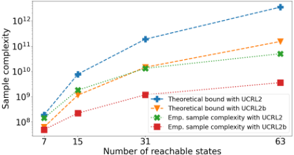
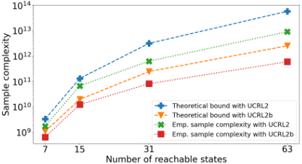
We use either UCRL2 [Jaksch et al., 2010] or UCRL2b [Fruit et al., 2020] as a black-box subroutine for METAEXPLORE. The problem settings used in the experiments are described in Table 1. All the results shown in this article are averaged over 100 independent runs. Figure 1 shows the empirical sample complexity for META-EXPLORE for problem setting 1 using δ = 0.2 and ϵ = 2/3. Figure 2 shows the empirical sample complexity for META-EXPLORE for problem setting 2 using δ = 0.1 and ϵ = 1/3. For each value of the number of reachable states shown in Figure 1 and 2, both the instantiations of META-EXPLORE were able to find appropriate output policies for corresponding reachable states in at least 1-δ fraction of the runs. In the appendix given with the extended version of this article, we provide additional experimental results.
The experimental results show that, using an appropriate RL algorithm as a black-box, our algorithm explores the state space properly. For both the theoretical upper bound and the empirical sample complexity, META-EXPLORE using UCRL2b shows better dependence on L than METAEXPLORE using UCRL2 which corroborates the dependence proven in Theorem 1. We also note, in general, for higher values of the number of reachable states (i.e., higher values of L), the empirical sample complexity tends to be much better than the sample complexity promised by the theoretical upper bounds. This further provides a testimony for our approach which is better able to leverage knowledge gained from solving simpler problems (i.e., smaller values of L) in order to solve more difficult problems efficiently. It also points to a way of improving the empirical performance of our approach in scenarios where solutions for simpler problems are known and can be provided to the algorithm which will in turn use them to find solutions for difficult problems in an efficient manner.
| Setting | P0,l | P0,m | P0,r | P1,l | P1,m | P1,r |
|---|---|---|---|---|---|---|
| Setting 1 | 0.90 | 0.050 | 0.050 | 0.050 | 0.050 | 0.90 |
| Setting 2 | 0.95 | 0.025 | 0.025 | 0.025 | 0.025 | 0.95 |
6 Concluding Remarks
We considered the problem of autonomous exploration in an unknown stationary environment. Our proposed algorithm can use any online RL algorithm (with appropriate regret guarantees) as a black-box to solve the relevant sub-tasks. We proved an upper bound on its sample complexity in terms of the regret bound of the used black-box RL algorithm. Our experimental results demonstrate the applicability of our proposed algorithm for the considered problem and the correctness of our theoretical results.
Interesting directions for future work include: 1) extending the problem definition to include non-stationary environments, 2) extending the solution approach to solve the multi-goal stochastic shortest path problem introduced by [Cai et al., 2022].
Acknowledgments
This work is supported by the Dutch Research Council (NWO) in the framework of the TEPAIV research project (project number 612.001.752) and the Austrian Science Fund (FWF): TAI 590-N.
@inproceedings{ijcai2023p413,
  title     = {Autonomous Exploration for Navigating in MDPs Using Blackbox RL Algorithms},
  author    = {Gajane, Pratik and Auer, Peter and Ortner, Ronald},
  booktitle = {Proceedings of the Thirty-Second International Joint Conference on
               Artificial Intelligence, {IJCAI-23}},
  publisher = {International Joint Conferences on Artificial Intelligence Organization},
  editor    = {Edith Elkind},
  pages     = {3714--3722},
  year      = {2023},
  month     = {8},
  note      = {Main Track},
  doi       = {10.24963/ijcai.2023/413},
  url       = {https://doi.org/10.24963/ijcai.2023/413},
}
TY - CPAPER TI - Autonomous Exploration for Navigating in MDPs Using Blackbox RL Algorithms AU - Gajane, Pratik AU - Auer, Peter AU - Ortner, Ronald T2 - Proceedings of the Thirty-Second International Joint Conference on Artificial Intelligence, IJCAI-23 PB - International Joint Conferences on Artificial Intelligence Organization PY - 2023 SP - 3714 EP - 3722 DO - 10.24963/ijcai.2023/413 UR - https://doi.org/10.24963/ijcai.2023/413 ER -Copied
Machine-readable versions of this paper, for tools and AI agents:





