
A Unification Framework for Euclidean and Hyperbolic Graph Neural Networks
Proceedings of the Thirty-Second International Joint Conference on Artificial Intelligence. Main Track. Pages 3875-3883.
https://doi.org/10.24963/ijcai.2023/431
Keywords
- Machine Learning: ML: Representation learning
- Machine Learning: ML: Sequence and graph learning
Abstract
Hyperbolic neural networks can effectively capture the inherent hierarchy of graph datasets, and consequently a powerful choice of GNNs. However, they entangle multiple incongruent (gyro-)vector spaces within a layer, which makes them limited in terms of generalization and scalability.
In this work, we propose the Poincaré disk model as our search space, and apply all approximations on the disk (as if the disk is a tangent space derived from the origin), thus getting rid of all inter-space transformations. Such an approach enables us to propose a hyperbolic normalization layer and to further simplify the entire hyperbolic model to a Euclidean model cascaded with our hyperbolic normalization layer. We applied our proposed nonlinear hyperbolic normalization to the current state-of-the-art homogeneous and multi-relational graph networks. We demonstrate that our model not only leverages the power of Euclidean networks such as interpretability and efficient execution of various model components, but also outperforms both Euclidean and hyperbolic counterparts on various benchmarks. Our code is made publicly available at https://github.com/oom-debugger/ijcai23.
- [Anderson and May, 1992] Roy M Anderson and Robert M May. Infectious diseases of humans: dynamics and con- trol. Oxford university press, 1992.
- [Balažević et al., 2019] Ivana Balažević, Carl Allen, and Timothy Hospedales. Multi-relational poincaré graph em- beddings. In Advances in Neural Information Processing Systems, 2019.
- [Becigneul and Ganea, 2019] Gary Becigneul and Octavian- Eugen Ganea. Riemannian adaptive optimization methods. In International Conference on Learning Representations, 2019.
- [Bordes et al., 2013] Antoine Bordes, Nicolas Usunier, Alberto Garcia-Duran, Jason Weston, and Oksana Yakhnenko. Translating embeddings for modeling multi-relational data. Advances in neural information processing systems, 26, 2013.
- [Cao et al., 2015] Shaosheng Cao, Wei Lu, and Qiongkai Xu. Grarep: Learning graph representations with global structural information. In Proceedings of the 24th ACM in- ternational on conference on information and knowledge management, pages 891-900, 2015.
- [Cayton, 2005] Lawrence Cayton. Algorithms for manifold learning. Univ. of California at San Diego Tech. Rep, 12(1- 17):1, 2005.
- [Chami et al., 2019] Ines Chami, Zhitao Ying, Christopher Ré, and Jure Leskovec. Hyperbolic graph convolutional neural networks. In Advances in Neural Information Pro- cessing Systems, pages 4869-4880, 2019.
- [Chen et al., 2020] Ming Chen, Zhewei Wei, Zengfeng Huang, Bolin Ding, and Yaliang Li. Simple and deep graph convolutional networks. In Hal Daumé III and Aarti Singh, editors, Proceedings of the 37th International Con- ference on Machine Learning, volume 119 of Proceedings of Machine Learning Research, pages 1725-1735. PMLR, 13-18 Jul 2020.
- [Chen et al., 2021] Boli Chen, Yao Fu, Guangwei Xu, Pengjun Xie, Chuanqi Tan, Mosha Chen, and Liping Jing. Probing bert in hyperbolic spaces. arXiv preprint arXiv:2104.03869, 2021.
- [Choudhary et al., 2021] Nurendra Choudhary, Nikhil Rao, Sumeet Katariya, Karthik Subbian, and Chandan K. Reddy. Self-supervised hyperboloid representations from logical queries over knowledge graphs. In Proceedings of the Web Conference 2021, WWW '21, page 1373-1384, 2021.
- [Choudhary et al., 2022] Nurendra Choudhary, Nikhil Rao, Sumeet Katariya, Karthik Subbian, and Chandan K. Reddy. Anthem: Attentive hyperbolic entity model for product search. In Proceedings of the Fifteenth ACM In- ternational Conference on Web Search and Data Mining, WSDM '22, page 161-171, New York, NY, USA, 2022. Association for Computing Machinery. [
- [Dettmers et al., 2018] Tim Dettmers, Pasquale Minervini, Pontus Stenetorp, and Sebastian Riedel. Convolutional 2d knowledge graph embeddings. In Proceedings of the AAAI conference on artificial intelligence, volume 32, 2018.
- [Fefferman et al., 2016] Charles Fefferman, Sanjoy Mitter, and Hariharan Narayanan. Testing the manifold hypoth- esis. Journal of the American Mathematical Society, 29(4):983-1049, 2016.
- [Fu et al., 2020] Xinyu Fu, Jiani Zhang, Ziqiao Meng, and Irwin King. Magnn: Metapath aggregated graph neural network for heterogeneous graph embedding. In WWW, 2020.
- [Ganea et al., 2018] Octavian Ganea, Gary Bécigneul, and Thomas Hofmann. Hyperbolic neural networks. In Ad- vances in neural information processing systems, pages 5345-5355, 2018.
- [Grover and Leskovec, 2016] Aditya Grover and Jure Leskovec. node2vec: Scalable feature learning for networks. In Proceedings of the 22nd ACM SIGKDD international conference on Knowledge discovery and data mining, pages 855-864, 2016.
- [Hamilton et al., 2017] William L. Hamilton, Rex Ying, and Jure Leskovec. Inductive representation learning on large graphs. In NIPS'17, 2017.
- [Ioffe and Szegedy, 2015] Sergey Ioffe and Christian Szegedy. Batch normalization: Accelerating deep net- work training by reducing internal covariate shift. In International conference on machine learning, pages 448-456. PMLR, 2015.
- [Kipf and Welling, 2017] Thomas N. Kipf and Max Welling. Semi-supervised classification with graph convolutional networks. In 5th International Conference on Learning Representations, ICLR 2017, Toulon, France, April 24-26, 2017, Conference Track Proceedings. OpenReview.net, 2017.
- [Krioukov et al., 2010] Dmitri Krioukov, Fragkiskos Pa- padopoulos, Maksim Kitsak, Amin Vahdat, and Marián Boguná. Hyperbolic geometry of complex networks. Physical Review E, 82(3):036106, 2010.
- [Lee, 2018] John M Lee. Introduction to Riemannian mani- folds, volume 176. Springer, 2018.
- [Lei Ba et al., 2016] Jimmy Lei Ba, Jamie Ryan Kiros, and Geoffrey E. Hinton. Layer Normalization. arXiv e-prints, page arXiv:1607.06450, July 2016.
- [Li et al., 2018] Qimai Li, Zhichao Han, and Xiao-Ming Wu. Deeper insights into graph convolutional networks for semi-supervised learning. In Thirty-Second AAAI confer- ence on artificial intelligence, 2018.
- [Narayanan et al., 2017] Annamalai Narayanan, Mahinthan Chandramohan, Rajasekar Venkatesan, Lihui Chen, Yang Liu, and Shantanu Jaiswal. graph2vec: Learning distributed representations of graphs. arXiv preprint arXiv:1707.05005, 2017.
- [Paszke et al., 2019] Adam Paszke, Sam Gross, Francisco Massa, Adam Lerer, James Bradbury, Gregory Chanan, Trevor Killeen, Zeming Lin, Natalia Gimelshein, Luca Antiga, et al. Pytorch: An imperative style, high- performance deep learning library. Advances in neural in- formation processing systems, 32:8026-8037, 2019.
- [Peng et al., 2021] Wei Peng, Tuomas Varanka, Abdelrah- man Mostafa, Henglin Shi, and Guoying Zhao. Hyper- bolic deep neural networks: A survey. arXiv preprint arXiv:2101.04562, 2021.
- [Rossi and Ahmed, 2015] Ryan A. Rossi and Nesreen K. Ahmed. The network data repository with interactive graph analytics and visualization. In AAAI, 2015.
- [Salimans and Kingma, 2016] Tim Salimans and Diederik P. Kingma. Weight normalization: A simple reparameteriza- tion to accelerate training of deep neural networks. In Pro- ceedings of the 30th International Conference on Neural Information Processing Systems, NIPS'16, page 901-909, Red Hook, NY, USA, 2016.
- Curran Associates Inc. [Scarselli et al., 2008]
- Franco Scarselli, Marco Gori, Ah Chung Tsoi, Markus Hagenbuchner, and Gabriele Monfardini. The graph neural network model. IEEE transactions on neural networks, 20(1):61-80, 2008.
- [Schlichtkrull et al., 2018] Michael Schlichtkrull, Thomas N Kipf, Peter Bloem, Rianne van den Berg, Ivan Titov, and Max Welling. Modeling relational data with graph convo- lutional networks. In European semantic web conference, pages 593-607. Springer, 2018.
- [Sen et al., 2008] Prithviraj Sen, Galileo Mark Namata, Mustafa Bilgic, Lise Getoor, Brian Gallagher, and Tina Eliassi-Rad. Collective classification in network data. AI Magazine, 29(3):93-106, 2008.
- [Shimizu et al., 2021] Ryohei Shimizu, YUSUKE Mukuta, and Tatsuya Harada. Hyperbolic neural networks++. In International Conference on Learning Representations, 2021.
- [Sun et al., 2019] Zhiqing Sun, Zhi-Hong Deng, Jian-Yun Nie, and Jian Tang. Rotate: Knowledge graph embedding by relational rotation in complex space. In International Conference on Learning Representations, 2019.
- [Thanapalasingam et al., 2021] Thiviyan Thanapalasingam, Lucas van Berkel, Peter Bloem, and Paul Groth. Rela- tional graph convolutional networks: A closer look, 2021. arXiv:2107.10015.
- [Toutanova et al., 2015] Kristina Toutanova, Danqi Chen, Patrick Pantel, Hoifung Poon, Pallavi Choudhury, and Michael Gamon. Representing text for joint embedding of text and knowledge bases. In Proceedings of the 2015 conference on empirical methods in natural language pro- cessing, pages 1499-1509, 2015.
- [Ungar, 2009] Abraham Albert Ungar. A Gyrovector Space Approach to Hyperbolic Geometry. Synthesis Lectures on Mathematics & Statistics. Morgan & Claypool Publishers, 2009.
- [Vaswani et al., 2017] Ashish Vaswani, Noam Shazeer, Niki Parmar, Jakob Uszkoreit, Llion Jones, Aidan N Gomez, Łukasz Kaiser, and Illia Polosukhin. Attention is all you need. In Advances in neural information processing sys- tems, pages 5998-6008, 2017.
- [Veličković et al., 2018] Petar Veličković, Guillem Cucurull, Arantxa Casanova, Adriana Romero, Pietro Liò, and Yoshua Bengio. Graph Attention Networks. International Conference on Learning Representations, 2018. accepted as poster.
- [Vyas et al., 2022] Anoushka Vyas, Nurendra Choudhary, Mehrdad Khatir, and Chandan K. Reddy. Graphzoo: A development toolkit for graph neural networks with hyper- bolic geometries. In Companion Proceedings of the Web Conference 2022, WWW '22, page 184-188, New York, NY, USA, 2022. Association for Computing Machinery.
- [Yang et al., 2015] Bishan Yang, Wen-tau Yih, Xiaodong He, Jianfeng Gao, and Li Deng. Embedding entities and relations for learning and inference in knowledge bases. In 3rd International Conference on Learning Representa- tions, ICLR, 2015.
- [Yang et al., 2021] Tianchi Yang, Linmei Hu, Chuan Shi, Houye Ji, Xiaoli Li, and Liqiang Nie. Hgat: Heteroge- neous graph attention networks for semi-supervised short text classification. ACM Transactions on Information Sys- tems (TOIS), 39(3):1-29, 2021.
- [Zhang et al., 2021] Yiding Zhang, Xiao Wang, Chuan Shi, Xunqiang Jiang, and Yanfang Fanny Ye. Hyperbolic graph attention network. IEEE Transactions on Big Data, pages 1-1, 2021.
References were extracted automatically from the PDF and may contain errors.
Full text extracted automatically from the PDF; figures, tables and equations may differ. The PDF is the version of record.
1 Introduction
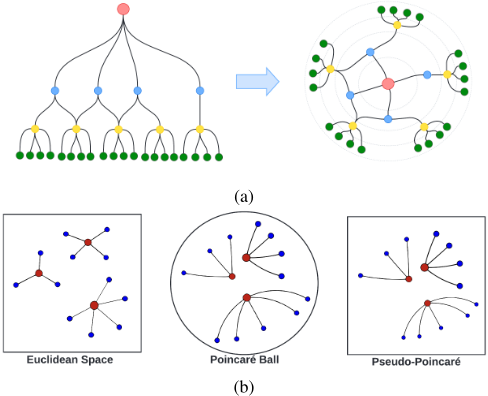
Graph data structures are ubiquitous. There have been several advancements in graph processing techniques across several domains such as citation networks [Sen et al., 2008], medicine [Anderson and May, 1992], and e-commerce [Choudhary et al., 2022]. Recently, non-Euclidean geometries such as hyperbolic spaces have shown significant potential in representation learning and graph prediction [Chami et al., 2019; Choudhary et al., 2021]. Due to their exponential growth in volume with respect to radius [Krioukov et al., 2010], hyperbolic spaces are able to embed hierarchical structures with low distortion, i.e., an increase in the number of nodes in a tree with increasing depth is analogous to moving outwards from the origin in a Poincar´e ball (since both grow exponentially). This similarity enables the hyperbolic space to project the child nodes exponentially further away from the origin compared to their parents (as shown in Figure
1.a) which captures hierarchy in the embedding space. There are certain fundamental questions about hyperbolic models which are yet to be studied. For example, hyperbolic models operate on completely new manifolds with their own gyrovector space [Ungar, 2009] (to be differentiated from the Euclidean vector space). Because they operate in a different manifold, techniques such as dropout or L1/2 regularization do not guarantee similar behavior. Moreover, while existing hyperbolic operations [Ganea et al., 2018] provide fair support for basic sequential neural networks, a correct translation of more complex Euclidean architectures (such as multiheaded attention networks [Vaswani et al., 2017]) is nontrivial and counter-intuitive, due to the special properties of Riemannian manifold [Shimizu et al., 2021]. Finally, hyperbolic operators are computationally expensive i.e., the number of complex mathematical operations for each primitive operator limits their scalability compared to the Euclidean graph neural networks.
Traditionally, hyperbolic models use a mixture of hyperbolic geodesics, gyro-vector space mathematics (e.g. Poincar´e disc model combined with M¨obius operations), and tangent space approximations at various points. Instead of switching between multiple frameworks with potentially incongruent operations, in this work, we let the Poincar´e disk model be our search space and propose to apply all approximations inplace on the Poincar´e disk (i.e., to apply all tangent space approximations on the disk as if the disk is a tangent space derived from the origin). This enables us to replace non-scalable gyro-vector/M¨obius operations with a Euclidean approximation, and then simplify the whole hyperbolic model as a Euclidean model cascaded with a hyperbolic normalization function. In our approach, we replace all M¨obius operations with Euclidean operations, yet we still work in the Riemannian manifold (by using our proposed hyperbolic normalization layer along with using Riemannian optimizer), thus, we call it Pseudo-Poincar´e framework (figure 1.b).
With our formulations, the trainable parameters lie in the Euclidean space, hence we can re-use the architectures that already exist for Euclidean solution space. This leads to the use of inexpensive operators. It also enables the use of existing well-optimized Euclidean models along with their hyperparameter settings tuned for specific tasks. Having the aforementioned two capabilities, our framework brings the best of two worlds together. For further evidence, we have applied our formulation to construct new pseudo-Poincar´e variants of GCN [Kipf and Welling, 2017], GAT [Veliˇckovi´c et al., 2018], and multi-relational graph embedding model MuR [Balaˇzevi´c et al., 2019], RGCN [Schlichtkrull et al., 2018] and GCNII [Chen et al., 2020] (we call our variants as NGCN, NGAT, NMuR, NRGCN, and NGCNII, respectively). We demonstrate that the reformulated variants outperform several state-of-the-art graph networks on standard graph tasks. Furthermore, our experiments indicate that our pseudo-Poincar´e variants benefit from using regularization methods used in Euclidean counterparts (unlike the traditional hyperbolic counterparts). We also show the execution speed of our proposed model to be comparable to that of the Euclidean counterparts and hence provide insights for building deeper hyperbolic (pseudo-Poincar´e) models.
2 RelatedWork
Research into graph representation learning can be broadly classified into two categories based on the nature of the underlying graph dataset: (i) Homogeneous graphs - where the edges connect the nodes but do not have any underlying information and (ii) Heterogeneous or multi-relational graphs - where the edges contain information regarding the type of connection or a complex relation definition. Early research in this area relied on capturing information from the adjacency matrix through factorization and random walks. In matrix factorization-based approaches [Cao et al., 2015], the adjacency matrix A is factorized into low-dimensional dense matrices L such that ∥LT L - A∥ is minimized. In random walk-based approaches [Grover and Leskovec, 2016; Narayanan et al., 2017], the nodes' information is aggregated through message passing over its neighbors through random or metapath traversal [Fu et al., 2020]. More recently, the focus has shifted towards neighborhood aggregation through neural networks, specifically, Graph Neural Networks (GNNs) [Scarselli et al., 2008]. In this line of work, several architectures such as GraphSage [Hamilton et al., 2017], GCN [Kipf and Welling, 2017], and GAT [Veliˇckovi´c et al., 2018] have utilized popular deep learning frameworks to aggregate information from the nodes' neighborhood. Concurrently multi-relational graph neural networks have been developed focusing on representation learning in knowledge graphs in which the nodes/entities can have edges/relations of different types. TransE [Bordes et al., 2013], DistMult [Yang et al., 2015], RotatE [Sun et al., 2019], MuRE [Balaˇzevi´c et al., 2019], RGCN [Schlichtkrull et al., 2018] are examples of multi-relational GNNs.
3 Hyperbolic Networks
Manifold hypothesis suggests that high dimensional data tends to lie in the vicinity of a low dimensional manifold [Cayton, 2005][Fefferman et al., 2016]. For such data, the model in fact learns the manifold to better learn the relation between the data points. In graph datasets, hierarchical structures are common, which tend to better align in hyperbolic manifolds. Using the aforementioned concept, Ganea, et al. [Ganea et al., 2018] proposed hyperbolic neural networks. Such a network operates in hyperbolic manifolds, simplifies the search space by omitting the manifold learning process, and thus, results in more efficient models for graph applications. That work led to several architectures for representation learning in both homogeneous (HGCN [Chami et al., 2019], HAT [Zhang et al., 2021]) and heterogeneous (MuRP [Balaˇzevi´c et al., 2019], HypE [Choudhary et al., 2021]) graph datasets. These architectures primarily utilize the gyrovector space model to formulate the neural network operations.
Hyperbolic space is a Riemannian manifold with constant negative curvature. The coordinates in the hyperbolic space can be represented in several isometric models such as Beltrami-Klein Model Knc and Poincar´e Ball Bnc . In this paper, we consider the Poincar´e Ball model because it is the most widely used one for hyperbolic networks. In a Poincar´e ball of curvature c, simple operations such as vector addition and scaling are done using M¨obius operation (addition ⊕c, scalar multiplication ⊗c). More complex operations such as aggregation, convolution, and attention are done in local tangent spaces which require transformation between Euclidean and hyperbolic space. For an embedding vector x ∈ Rn from point v, its corresponding hyperbolic embedding in the Poincar´e ball of curvature c, p ∈ Bnc is calculated with the exponential map as:
where λ is the conformal factor at point v. Conversely, logarithmic map is used to transform a hyperbolic embedding p ∈ Bnc to a Euclidean vector x ∈ Rn is formulated as:
Note that the tangent space approximation relies on the assumption of spatial locality (i.e., small vectors starting from point v). For transporting a local vector from a point in the Hyperbolic manifold to another point, one can use parallel transport [Lee, 2018]. Parallel transport is specifically used in bias addition in Hyperbolic linear layers [Chami et al., 2019]. For a detailed discussion on parallel transport, please refer to [Lee, 2018].
4 Pseudo-Poincar´e Hyperbolic Networks
While hyperbolic networks show promising results, switching back and forth between M¨obius gyro-vector operations and Euclidean tangent approximations (at various points) makes them computationally expensive, limits their extensibility, and makes them less predictable when applying L1/2 regularization and dropout. Furthermore, such back and forth between the manifolds (at variable points) comes with an implicit assumption that the embeddings have spatial locality in all dimensions for the models to be performant. We argue that approximating on tangent space at a variable point does not necessarily increase the approximation accuracy because the spatial locality of the embeddings is not guaranteed in general. Therefore, fixating tangent space to be at the origin can bring both simplicity to the model and performance in general cases. Moreover, only tangent space at origin has a one-to-one mapping with all points on the Poincar´e (hyperbolic) half-plane model. This enables us to combine the tangent space approximation with Poincar´e half-plane model and apply all approximations in the half-plane. This makes the pseudo-Poincar´e networks much easier to understand, develop, and optimize. Fixating the tangent space to the point of origin simplifies the exponential maps (eq. 1) as:
Conversely, the logarithmic map (eq. 2) is simplified as:
Using Eq. (3) and Eq. (4), we reformulate the hyperbolic feed-forward layer. In this section, we only discuss the reformulation for Pseudo-Poincar´e Feed-forward Layer. The convolution, attention, and multi-relation layer can be similarly reformulated for the Pseudo-Poincar´e paradigm.
Pseudo-Poincar´e Feed-forward Layer. We state that cascading hyperbolic feed-forward layers (including linear layers) is equivalent to cascading their Euclidean counterparts and then applying a hyperbolic normalization to the result.
Lemma 1. For a point in the tangent space at origin x ∈ T0n Bnc , the exponential map to the hyperbolic space Bnc , expc0 : T0n Bnc → Bnc expc0 (x), is equivalent to the input scaled by a non-linear scalar function ω : Rn → Rn , i.e.,
where ω(x) is the hyperbolic normalization for exponential maps. This follows from equation (1).
Lemma 2. Let f ⊗c be a single hyperbolic feed-forward layer, and f ⊗c be its euclidean counterpart. Approximating on tangent space at origin for all stages makes the cascade of n hyperbolic feed-forward layers F ⊗c n = {f ⊗c i }ni=1 to be equivalent to cascading n of their Euclidean counterparts Fn = {fi}ni=1 encapsulated in logc0 and expc0 functions, i.e.,
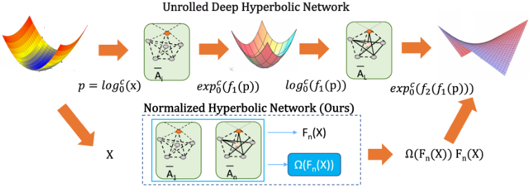
Proposition Lemma 2 implies that the hyperbolic transformations expc0 and logc0 are only needed at the initial and final stages to capture hierarchy in Euclidean networks.
Lemma 3. For given input features x = logc0 (p) ∈ Rn , a given hyperbolic feed forward layer can be rewritten as f ⊗c (x) := ω(f(x))f(x).
From lemmas 2 and 3, we arrive at the following theorem for cascaded hyperbolic layers.
Theorem 4. Fixating the tangent space to be always at origin, cascaded hyperbolic feed-forward layers F ⊗c n for Euclidean input x ∈ Rn can be reformulated as F ⊗c n (x) :=
Ω(Fn(x))Fn(x), where Ω(Fn(x)) is the hyperbolic normalization for a cascaded hyperbolic feed-forward network. Note that ω() is the exponential transformation factor at the variable level and Ω() is the same at the level of neural networks.
Hyperbolic Normalization. Theorem 4 allows the cascaded hyperbolic layers to be reformulated in the Euclidean space using a hyperbolic normalization (Ω) function. Our normalization layer resembles the technique proposed in [Salimans and Kingma, 2016] to normalize the weights, which uses the equation; w = es ∥v∥ v, where v is an n-dimensional vector used to learn the direction and s is a trainable parameter. However, unlike weight normalization, hyperbolic normalization happens on the features (and not the weights). Furthermore, hyperbolic normalization uses the tanh scaling function instead of es . However, both are similar in terms of using the feature vector magnitude as the denominator and hence removing the orthogonality of the dimensions. The "unrolled deep hyperbolic network" (shown in Figure 2) presents the general idea of stacking multiple hyperbolic layers together. The input into each layer is passed through a logarithmic map to project into Euclidean space and its output is projected back onto the hyperbolic space after applying the computations.
Batch-Norm, Layer-Norm vs. Hyperbolic Norm. BatchNorm tries to reduce the covariant shift and noise [Ioffe and Szegedy, 2015] which means the result of the batch-norm is in Euclidean space. On the other hand, Layer-Norm, and Hyperbolic Norm take vectors to another manifold for better latent space representation [Lei Ba et al., 2016]. Thus, we recommend using Riemannian optimizers when applying our method at least for shallow GNNs (we provided empirical results in the next section). Note that, in order to apply the batch normalization in hyperbolic space, one needs to change its mathematical operations to use Frechet mean [Peng et al., 2021]. The detailed analysis of the effect of hyperbolic batch normalization is outside the scope of this work.
Optimization. The scaling function in Eq. (5) uses the vector norm in the denominator and hence, each dimension depends on the value of other dimensions (i.e., nonorthogonal). Due to this, optimizers that are developed based on the orthogonality assumptions of the dimensions such as ADAM are not expected to produce the most optimal weights. Thus, we choose Riemannian optimizers such as Riemannian ADAM [Becigneul and Ganea, 2019] for our model training. For traditional hyperbolic models, regularization techniques such as L2-regularization do not work as expected since the weights are in hyperbolic space. However, the trainable parameters in our formulation are in the Euclidean space. Hence, we can additionally apply regularization techniques that are applied to Euclidean networks.
5 Experimental Setup
In this section, we aim to answer the following research questions (RQs) through our experiments:
RQ1: How do the pseudo-Poincar´e variants compare to their Euclidean and hyperbolic counterparts on node classification and link prediction?
RQ2: How does the pseudo-Poincar´e variant, NMuR, compare to its Euclidean and hyperbolic counterparts on reasoning over knowledge graphs?
RQ3: How do pseudo-Poincar´e variants react to the choice of optimizers, and what are the effects on their execution time? How does hyperbolic normalization compare to its counterparts?
RQ4: How does pseudo-Poincar´e variant perform when used in deep GNN architectures?
5.1 Experimental Setup
For comparison of hyperbolic normalization with other methods, we conduct our experiments on the following tasks: (i) graph prediction (node classification and link prediction) and (ii) reasoning over knowledge graphs, described below:
Graph Prediction. Given a graph G = (V × E), where vi ∈ Rn , {vi}|V | i=1 ∈ V is the set of all nodes and E ∈ {0, 1}|V |×|V | is the Boolean adjacency matrix, where |V | is the number of nodes in the graph and eij = 1, if link exists between node i and j, and eij = 0, otherwise. Each node vi ∈ V is also labeled with a class yi. In the task of node classification, the primary aim is to estimate a predictor model Pθ with parameters θ such that for an input node vi; Pθ(vi|E) = yi. In the task of link prediction, the primary aim is to estimate a predictor model Pθ with parameters θ such that for an input node-pair vi, vj and an incomplete adjacency matrix ˆE; Pθ(vi, vj | ˆE) = eij , where eij ∈ E is an element in the complete adjacency matrix.
Reasoning over Knowledge Graphs. Let us say that a set of triplets constitutes a knowledge graph KG = {(hi, ri, ti)}|KG| i=1 , where hi ∈ Rn and ti ∈ Rn are the head and tail entity, respectively connected by a relation ri ∈ Rn . In the task of reasoning [Balaˇzevi´c et al., 2019], our goal is to learn representations for the entities and relations using a scoring function that minimizes the distance between heads and tails using the relation as a transformation. We use the same formulation as [Balaˇzevi´c et al., 2019].
5.2 Datasets and Baselines
Datasets. For comparing our model with the baselines, we chose the following standard benchmark datasets; Cora [Rossi and Ahmed, 2015] contains 2708 publications with paper and author information connected by citation links and classified into 7 classes based on their research areas, Pubmed [Sen et al., 2008] contains medical publications pertaining to diabetes labeled into 3 classes. The dataset is collected from the Pubmed database, Citeseer [Sen et al., 2008] contains 3312 annotated scientific publications connected by citation links and classified into 6 classes of research areas, WN18RR [Dettmers et al., 2018] is a subset of the hierarchical WordNet relational graph that connects words with different types of semantic relations. WN18RR consists of 40,943 entities connected by 11 different semantic relations and FB15k-237 [Bordes et al., 2013] [Toutanova et al., 2015] contains triple relations of the knowledge graph and textual mentions from the Freebase entity pairs, with all simple invertible relations are removed for better comparison. The dataset contains 14,541 entities connected by 237 relations.
| Repr. | Datasets | Node Classification (Accuracy in%) | Link Prediction (ROC in%) | ||||
|---|---|---|---|---|---|---|---|
| Space | Models | CORA | Pubmed | Citeseer | Cora | Pubmed | Citeseer |
| Euclidean | GCN | 80.1±0.3 | 78.5±0.3 | 71.4±0.3 | 90.2±0.2 | 92.6±0.2 | 91.3±0.2 |
| GAT | 82.7±0.2 | 79.0±0.3 | 71.6±0.3 | 89.6±0.2 | 92.4±0.2 | 93.6±0.2 | |
| Hyperbolic | HGCN | 77.9±0.3 | 78.9±0.3 | 69.6±0.3 | 91.4±0.2 | 95.0±0.1 | 92.8±0.3 |
| HGAT | 79.6±0.3 | 79.2±0.3 | 68.1±0.3 | 90.8±0.2 | 93.9±0.2 | 92.2±0.2 | |
| Pseudo- | NGCN | 82.4±0.2 | 78.8±0.3 | 71.9±0.3 | 91.3±0.2 | 94.7±0.1 | 92.8±0.2 |
| Poincar´e | NGAT | 83.1±0.2 | 79.1±0.3 | 73.8±0.3 | 90.5±0.2 | 93.9±0.2 | 92.8±0.2 |
Protein-Protein Interaction (PPI) network dataset [Hamilton et al., 2017] contains 12M+ triples with 15 relations (preserving the original ratio of the relations in the dataset, we randomly sampled the dataset, and trained on the sampled subset). We use Cora, Pubmed, and Citeseer for our experiments on homogeneous graph prediction, i.e., node classification and link prediction. For comparing the multi-relational networks on the task of reasoning, we utilize the FB15k-237 and WN18RR datasets. For a fair comparison of evaluation metrics, we use the same training, validation, and test splits as used in the previous methods, i.e., the splits for Cora, Pubmed, and Citeseer are as given in [Chami et al., 2019] and for FB15k-237 and WN18RR, the splits are in accordance with [Balaˇzevi´c et al., 2019].
Baselines. For comparing the performance of our PseudoPoincar´e models, we utilize the Euclidean and hyperbolic variants of the architecture as our baselines; Graph Convolution (GCN) [Kipf and Welling, 2017] aggregates the message of a node's k-hop neighborhood using a convolution filter to compute the neighbor's significance to the root. Relational Graph Convolution Network (RGCN) [Schlichtkrull et al., 2018] is graph convolutional networks applied in heterogeneous graph. Deep Graph Convolutional Networks (GCNII) [Chen et al., 2020] is an extension of a Graph Convolution Networks with two new techniques, initial residual and identify mapping, to be used in deep GNN settings. Graph Attention (GAT) [Veliˇckovi´c et al., 2018] aggregates the messages from the neighborhood using learnable attention weights. Hyperbolic Graph Convolution (HGCN) [Chami et al., 2019] is a hyperbolic formulation of the GCN network that utilizes the hyperbolic space and consequently, M¨obius operations to aggregate hierarchical features from the neighborhood. Hyperbolic Graph Attention (HGAT) [Yang et al., 2021] is a hyperbolic formulation of the GAT networks to capture hierarchical features in the attention weights. Multirelational Embeddings (MuRE) [Balaˇzevi´c et al., 2019] transforms the head entity by a relation matrix and then learns representation by minimizing L1-norm between head and tail entities translated by the relation embedding. Multirelational Poincar´e (MuRP) [Balaˇzevi´c et al., 2019] is a hyperbolic equivalent of MuRE that transforms the head entity by a relation matrix in the Poincar´e ball and then learns representation by minimizing the hyperbolic distance between the head and tail entities translated by the relation embedding.
5.3 Implementation Setup
Our models are implemented on the Pytorch framework [Paszke et al., 2019] and the baselines are adopted from [Chami et al., 2019; Vyas et al., 2022] for GAT, GCN, and HGCN, and from [Balaˇzevi´c et al., 2019] for MuRE and MuRP. Due to the unavailability of a public implementation, we use our own implementation of HGAT based on [Yang et al., 2021]. The implementations have been thoroughly tuned with different hyper-parameter settings for the best performance. For GAT baseline, we used 64 dimensions with 4 and 8 attention heads (we found 4 heads perform better and hence we only present that result in our tables), with dropout rate of 0.6 and L2 regularization of λ = 0.0005 (for Pubmed and Cora), and λ = 0.001 (for CiteSeer) to be inline with the hyper-parameters reported in [Veliˇckovi´c et al., 2018]. We used same number of dimensions and hyper-parameters for our NGAT model. For GCN baseline, [Veliˇckovi´c et al., 2018] used 64 dimensions. we used the same number of dimensions and hyperparameter setting as GAT baseline. It should be noted that, we observed poor performance when we applied regularization techniques (that GAT baseline used) to the hyperbolic models. For HGCN, the original paper used 16 hidden dimension, however, we tried 64, 32, and 16 for the hidden dimensions, we found 64 dimensions produces better results. For the curvature choice, we used different curvatures for different tasks. For the task of node classification, we used c = 0.3 (for Cora), and c = 1 (for Pubmed and Citeseer) as they produced the best results, while for the link prediction task, c = 1.5 produced the best results.
5.4 RQ1: Performance on Graph Prediction
To evaluate the performance of hyperbolic normalization with respect to Euclidean and hyperbolic alternatives, we compare NGCN and NGAT models against the baselines on node classification and link prediction. We utilize the standard evaluation metrics of accuracy and ROC-AUC for node classification and link prediction, respectively (Table 1).
From the results, in all cases (except link-prediction on Citeseer), pseudo-Poincar´e variants outperform the Euclidean model. Pseudo-Poincar´e variants perform better than their hyperbolic counterparts in node classification, but marginally inferior in link prediction. This is inline with our expectations as embeddings of adjacent points in link prediction on homogeneous graphs tend to have spatial locality. However, the spatial locality is less likely for node classification (as far away nodes still can belong to the same class). It is also worth noting that Pseudo-Poincar´e outperforms Euclidean in all node-classification datasets regardless of the hyperbolicity of the dataset (e.g., Cora has low hyperbolicity [Chami et al., 2019] which was previously suggested as a reason that inferior Hyperbolic networks over Euclidean counterparts). This observation suggests that Pseudo-Poincar´e is a more generalpurpose framework (i.e., it is performant in a wider variety of tasks/datasets compared to the pure-Hyperbolic model). It should be noted that pseudo-Poincar´e variants are consistently at least the second-best performing methods, closely following the top performer which makes it appealing given the low complexity, and speedup of the model (Table 6).
| WN18RR | FB15K-237 | PPI | ||||||||
|---|---|---|---|---|---|---|---|---|---|---|
| DimModels | MRR | H@10 | H@3 | MRR | H@10 | H@3 | MRR | H@10 | H@3 | |
| 40 | MuRE | 40.9±0.3 | 49.7±0.3 | 44.5±0.3 | 29.0±0.3 | 46.2±0.3 | 31.9±0.3 | 2.81±0.3 | 9.24±0.3 | 4.11±0.3 |
| MuRP | 42.5±0.3 | 52.2±0.3 | 45.9±0.3 | 29.8±0.3 | 47.4±0.3 | 32.8±0.3 | 5.55±0.3 | 10.21±0.3 | 4.43±0.3 | |
| NMuR | 43.6±0.3 | 57.5±0.3 | 47.4±0.3 | 31.5±0.3 | 49.7±0.3 | 34.7±0.3 | 8.21±0.3 | 14.3±0.3 | 11.7±0.3 | |
| 200 | MuRE | 44±0.3 | 51.3±0.3 | 45.5±0.3 | 31.4±0.3 | 49.5±0.3 | 34.5±0.3 | 10.68±0.3 | 14.55±0.3 | 11.90±0.3 |
| MuRP | 44.6±0.3 | 52.4±0.3 | 46.2±0.3 | 31.5±0.3 | 49.8±0.3 | 34.8±0.3 | 8.23±0.3 | 15.09±0.3 | 9.98±0.3 | |
| NMuR | 44.7±0.3 | 57.9±0.3 | 48.1±0.3 | 32.2±0.3 | 50.6±0.3 | 35.5±0.3 | 12.68±0.3 | 15.07±0.3 | 13.82±0.3 | |
5.5 RQ2: Multi-relational Reasoning
To compare the performance of hyperbolic normalization against the baselines for multi-relational graphs, we compare the NMuR model against MuRE and MuRP on the task of reasoning. We consider the standard evaluation metrics of Hits@K and Mean Reciprocal Rank (MRR) to compare our methods on the reasoning task. Let us say that the set of results for a head-relation query (h, r) is denoted by R(h,k), then the metrics are computed by MRR = 1n ∑ni=1 1 rank(i) and Hits@K = 1K ∑Kk=1 ek, where ek = 1, if ek ∈ R(h,r) and 0, otherwise. Here rank(i) is the rank of the ith retrieved sample in the ground truth. To study the effect of dimensionality, we evaluate the models with two values of the embedding dimensions: n = 40 and n = 200. The results from our comparison are given in Table 2. From the results, note that NMuR outperforms the hyperbolic model MuRP, on average, by ≈ 5% with 40 dimensions and ≈ 3% with 200 dimensions across various metrics and datasets. This shows that NMuR is able to effectively learn better representations at a lower number of dimensions. Also, note that the difference in performance by increasing the number of dimensions is < 1% for most cases, implying that NMuR is already able to capture the hierarchical space of the knowledge graphs at lower dimensions. This should limit the memory needed for reasoning without a significant loss in performance.
Applying Pseudo-Poincare to RGCN
In order to further show (1) the effectiveness of our method, as well as (2) how easy it is to apply our method to an existing model (i.e., adaptability), we took the pytorch models implemented by [Thanapalasingam et al., 2021], and added our hyperbolic normalization layer as the last layer of the model.
| Dataset | AIFB | AM | BGS | MUTAG |
|---|---|---|---|---|
| RGCN | 97.22 | 89.39 | 82.76 | 67.65 |
| NRGCN | 97.22 | 89.9 | 89.66 | 73.53 |
| E-RGCN | 88.89 | 90.4 | 82.76 | 75.00 |
| NE-RGCN | 94.44 | 90.91 | 86.21 | 76.47 |
| Base Model | CR | PM | CS | |
|---|---|---|---|---|
| GCN | Constant | 67.9 | 76.7 | 68.3 |
| Layer-Norm | 78.3 | 75.0 | 63.6 | |
| Hyp-Norm | 80.9 | 78.0 | 72.1 | |
| GAT | Constant | 75.3 | 73.0 | 61.2 |
| Layer-Norm | 75.6 | 74.9 | 65.3 | |
| Hyp-Norm | 76.7 | 76.3 | 68.6 |
We also trained the model using Riemannian ADAM. Table 3 shows the comparative results for the Node Classification tasks on AIFB, AM, BGS, and MUTAG datasets (further details about the datasets can be found in [Thanapalasingam et al., 2021]). We used curvature c = 1.5, and scaling factor s = 3 for N-RGCN and c = 0.5, and s = 5 for NE-RGCN (except for MUTAG NE-RGCN that we used c = 1.5, and s = 3). We trained the models 10 times and picked the best checkpoint for both Euclidean and our variant. We observed significant improvements across all metrics when we applied our Hyperbolic normalization method. The fact that applying our method to the existing models is almost seamless increases the ability to explore/adopt hyperbolic models for a variety of tasks/models/applications.
5.6 RQ3: Model Analysis
Hyperbolic Normalization vs. Layer Normalization. In this experiment, we study the difference between our hyperbolic normalization compared to other existing normalization approaches. For this, we select Layer-norm [Lei Ba et al., 2016] as it is the closest in terms of input/output. Also, in order to study the effect of hyperbolic scaling in our normalization layer, we added constant-norm which is computed as follows: norm(x) = x/∥x∥. In order to compare the effect of normalization layers, we did not use any extra hyperparameter tuning and regularization. We set the embedding size to 64 for both GAT and GCN and used 4 heads for GAT models. Table 4 shows the comparison of different normalization methods on Cora, Pubmed, and Citeseer datasets, and confirms the outperformance of hyperbolic normalization. Since Layer-norm keeps the GAT model in the Euclidean space, we used ADAM optimizer. However, since both hyperbolic normalization and constant normalization have ∥x∥ as their denominator, we used Riemannian ADAM. Optimizer Choice. We experimentally validate our observations regarding the optimizer choice. Table 5 shows NGAT works better when Riemannian ADAM is used. This shows although the parameters are in Euclidean space, their gradient updates occur in accordance with hyperbolic gradients.
| Models | Optimizers | Cora | Pubmed | Citeseer |
|---|---|---|---|---|
| GAT | ADAM 82.7±0.2 | 78.7±0.2 | 71.6±0.3 | |
| RADAM 78.4±0.3 | 79.0±0.3 | 71.1±0.3 | ||
| HGAT | ADAM | 76.8±0.3 | 76.0±0.3 | 68.1±0.3 |
| RADAM | 79.6±0.3 | 78.9±0.3 | 68.1±0.3 | |
| NGAT | ADAM | 78.8±0.3 | 77.7±0.3 | 69.7±0.3 |
| RADAM | 83.9±0.2 | 79.1±0.3 | 73.8±0.3 |
| Model | CR | PM | CS | |
|---|---|---|---|---|
| Convolution | GCN | 0.07 | 0.13 | 0.04 |
| HGCN | 0.29 | 0.33 | 0.21 | |
| NGCN | 0.08 | 0.14 | 0.06 | |
| Attention | GAT | 0.16 | 0.38 | 0.09 |
| HGAT | 1.10 | 1.34 | 0.81 | |
| NGAT | 0.19 | 0.37 | 0.12 |
Execution Time Comparison. In this analysis, we demonstrate the impact of hyperbolic normalization in improving the scalability of hyperbolic networks. We study the computational cost to train our model versus the hyperbolic and Euclidean counterparts. We ran the following experiments on Quadro RTX 8000 with 48GB memory and reported the mean of epoch/second for each training experiment for the link prediction task in Table 6. Our model NGCN is 3 times faster than the HGCN on average over the entire training, while NGAT is 5 times faster than its own hyperbolic counterpart (HGAT). NGCN and NGAT are 25% and 12% slower compared to their Euclidean counterparts, respectively. We observed the smallest speedup for Pubmed which is due to the large dataset memory footprint. Note that for Pubmed our NGCN model is still more than 2 times faster than HGCN and NGAT is more than 3.5 times faster than HGAT.
5.7 RQ4: Hyperbolic Norm on Deep GNNs
[Li et al., 2018] indicates that traditional GNNs such as GCN and GAT achieve their best performance with 2-layer models. Stacking more layers and adding non-linearity tends to degrade the performance of these models. Such a phenomenon is called over-smoothing. So far, in our experiment, we showed that adding our hyperbolic normalization layer (plus Riemannian ADAM optimizer) increases the model performance. In order to understand the behavior of our layer on deep GNNs, we experimented on GCNII with 2, 4, 8, 16, 32, and 64 layers. It should be noted that, since our hyperbolic normalization layer contains tanh, adding the normalization layer to all GCNII causes a vanishing gradient problem. Thus, we only used our hyperbolic normalization layer in the middle of the model to form an encoder-decoder model (in which the encoder creates a hyperbolic latent space, and a normal decoder interprets the latent space). We picked the same Euclidean hyper-parameters as the original GCNII work [Chen et al., 2020] but did a grid search on curvature and scale. Table 7 shows the results for Cora, Citeseer, and Pubmed node classification tasks. As a general observation, the best pick (across models with different layers) of our normalized N-GCNII is either on par or outperforms the best pick of Euclidean GCNII. However, when we look more granular, we observe our model (N-GCNII), outperforms the Euclidean counterpart with better margin in the shallow models. As the number of layers increases, the performance gap reduces as well. We believe this is due to the fact that deeper models are better at learning smooth manifolds which is consistent with studies on NLP indicating the latent space of deep models shows a degree of hyperbolicity [Chen et al., 2021]. Moreover, we observed that as the model gets deeper, applying Riemannian ADAM is less effective, specifically, for models deeper than 8 layers, ADAM performs better even on our models.
| Models | 2 | 4 | 8 | 16 | 32 | 64 | |
|---|---|---|---|---|---|---|---|
| Cora | GCNII | 83.1 | 83.6 | 84.6 | 85.6 | 86.4 | 86.1 |
| NGCNII | 83.6 | 84.5 | 85.4 | 85.8 | 86.3 | 86.1 | |
| Citeseer | GCNII | 68.7 | 69.1 | 71.3 | 73.4 | 73 | 73.2 |
| NGCNII | 69.8 | 70.2 | 68.8 | 73.6 | 74.1 | 73.1 | |
| Pubmed | GCNII | 78.6 | 78.5 | 79 | 80.8 | 80.2 | 80.4 |
| NGCNII | 79.4 | 79.2 | 80 | 80.5 | 80.9 | 80.5 |
6 Conclusion
In this paper, we showed that a Euclidean model can be converted to behave as a hyperbolic model by simply (1) connecting it to the hyperbolic normalization layer and (2) using a Riemannian optimizer. From the training perspective, this approach allows the trainable parameters to interact in the Euclidean vector space, consequently enabling the use of Euclidean regularization techniques for the model training. Furthermore, the training of our proposed approach is significantly faster compared to the existing hyperbolic methods. This allows the hyperbolic networks to be more flexible in practice to a wider variety of graph problems. From task perspective, we removed the implicit assumption of having spatial locality of the adjacent nodes (in all dimensions), to be a prerequisite of the hyperbolic model training. This allows the framework to be applied on a wider range of tasks.
Acknowledgements
This work was supported in part by the Pacific Northwest National Laboratory (PNNL) through the Battelle Memorial Institute for the U.S. Department of Energy under Contract DE-AC05-76RL01830, and in part by the Data Model Convergence (DMC) Initiative at PNNL.
@inproceedings{ijcai2023p431,
  title     = {A Unification Framework for Euclidean and Hyperbolic Graph Neural Networks},
  author    = {Khatir, Mehrdad and Choudhary, Nurendra and Choudhury, Sutanay and Agarwal, Khushbu and Reddy, Chandan K.},
  booktitle = {Proceedings of the Thirty-Second International Joint Conference on
               Artificial Intelligence, {IJCAI-23}},
  publisher = {International Joint Conferences on Artificial Intelligence Organization},
  editor    = {Edith Elkind},
  pages     = {3875--3883},
  year      = {2023},
  month     = {8},
  note      = {Main Track},
  doi       = {10.24963/ijcai.2023/431},
  url       = {https://doi.org/10.24963/ijcai.2023/431},
}
TY - CPAPER TI - A Unification Framework for Euclidean and Hyperbolic Graph Neural Networks AU - Khatir, Mehrdad AU - Choudhary, Nurendra AU - Choudhury, Sutanay AU - Agarwal, Khushbu AU - Reddy, Chandan K. T2 - Proceedings of the Thirty-Second International Joint Conference on Artificial Intelligence, IJCAI-23 PB - International Joint Conferences on Artificial Intelligence Organization PY - 2023 SP - 3875 EP - 3883 DO - 10.24963/ijcai.2023/431 UR - https://doi.org/10.24963/ijcai.2023/431 ER -Copied
Machine-readable versions of this paper, for tools and AI agents:





