
Not Only Pairwise Relationships: Fine-Grained Relational Modeling for Multivariate Time Series Forecasting
Proceedings of the Thirty-Second International Joint Conference on Artificial Intelligence. Main Track. Pages 4416-4423.
https://doi.org/10.24963/ijcai.2023/491
Keywords
- Machine Learning: ML: Time series and data streams
- Data Mining: DM: Mining graphs
- Data Mining: DM: Mining spatial and/or temporal data
Abstract
Recent graph-based methods achieve significant success in multivariate time series modeling and forecasting due to their ability to handle relationships among time series variables. However, only pairwise relationships are considered in most existing works. They ignore beyond-pairwise relationships and their potential categories in practical scenarios, which leads to incomprehensive relationship learning for multivariate time series forecasting. In this paper, we present ReMo, a Relational Modeling-based method, to promote fine-grained relational learning among multivariate time series data. Firstly, by treating time series variables and complex relationships as nodes and hyperedges, we extract multi-view hypergraphs from data to capture beyond-pairwise relationships. Secondly, a novel hypergraph message passing strategy is designed to characterize both nodes and hyperedges by inferring the potential categories of relationships and further distinguishing their impacts on time series variables. By integrating these two modules into the time series forecasting framework, ReMo effectively improves the performance of multivariate time series forecasting. The experimental results on seven commonly used datasets from different domains demonstrate the superiority of our model.
- [Bai et al., 2020] Lei Bai, Lina Yao, Can Li, Xianzhi Wang, and Can Wang. Adaptive graph convolutional recurrent network for traffic forecasting. In NeurIPS, 2020.
- [Bai et al., 2021] Song Bai, Feihu Zhang, and Philip HS Torr. Hypergraph convolution and hypergraph attention. Pattern Recognition, 110:107637, 2021.
- [Binkowski et al., 2018] Mikolaj Binkowski, Gautier Marti, and Philippe Donnat. Autoregressive convolutional neural networks for asynchronous time series. In ICML, 2018.
- [Cao et al., 2020] Defu Cao, Yujing Wang, Juanyong Duan, Ce Zhang, Xia Zhu, Congrui Huang, Yunhai Tong, Bix- iong Xu, Jing Bai, Jie Tong, and Qi Zhang. Spectral temporal graph neural network for multivariate time-series forecasting. In NeurIPS, 2020.
- [Chen et al., 2021] Yuzhou Chen, Ignacio Segovia, and Yu- lia R Gel. Z-gcnets: time zigzags at graph convolutional networks for time series forecasting. In ICML, 2021.
- [Feng et al., 2019] Yifan Feng, Haoxuan You, Zizhao Zhang, Rongrong Ji, and Yue Gao. Hypergraph neural net- works. In AAAI, 2019.
- [Jang et al., 2017] Eric Jang, Shixiang Gu, and Ben Poole. Categorical reparameterization with gumbel-softmax. In ICLR, 2017.
- [Jin et al., 2018] Bo Jin, Haoyu Yang, Leilei Sun, Chuanren Liu, Yue Qu, and Jianing Tong. A treatment engine by predicting next-period prescriptions. In KDD, 2018.
- [Kipf et al., 2018] Thomas N. Kipf, Ethan Fetaya, Kuan- Chieh Wang, Max Welling, and Richard S. Zemel. Neu- ral relational inference for interacting systems. In ICML, 2018.
- [Lai et al., 2018] Guokun Lai, Wei-Cheng Chang, Yiming Yang, and Hanxiao Liu. Modeling long-and short-term temporal patterns with deep neural networks. In SIGIR, 2018.
- [Li et al., 2018] Yaguang Li, Rose Yu, Cyrus Shahabi, and Yan Liu. Diffusion convolutional recurrent neural net- work: Data-driven traffic forecasting. In ICLR, 2018.
- [Lim and Zohren, 2021] Bryan Lim and Stefan Zohren. Time-series forecasting with deep learning: a survey. Phi- los. Trans. Royal Soc. A, 379:20200209, 2021.
- [Maddison et al., 2017] Chris J. Maddison, Andriy Mnih, and Yee Whye Teh. The concrete distribution: A con- tinuous relaxation of discrete random variables. In ICLR, 2017.
- [Mudelsee, 2019] Manfred Mudelsee. Trend analysis of cli- mate time series: A review of methods. Earth-science re- views, 190:310-322, 2019.
- [Roberts et al., 2013] Stephen Roberts, Michael Osborne, Mark Ebden, Steven Reece, Neale Gibson, and Suzanne Aigrain. Gaussian processes for time-series modelling. Philos. Trans. Royal Soc. A, 371:20110550, 2013.
- [Shih et al., 2019] Shun-Yao Shih, Fan-Keng Sun, and Hung-yi Lee. Temporal pattern attention for multivari- ate time series forecasting. Machine Learning, 108:1421- 1441, 2019.
- [Sun et al., 2022] Fan-Yun Sun, Isaac Kauvar, Ruohan Zhang, Jiachen Li, Mykel Kochenderfer, Jiajun Wu, and Nick Haber. Interaction modeling with multiplex atten- tion. arXiv preprint arXiv:2208.10660, 2022.
- [Wu et al., 2019] Zonghan Wu, Shirui Pan, Guodong Long, Jing Jiang, and Chengqi Zhang. Graph wavenet for deep spatial-temporal graph modeling. In IJCAI, 2019. IJCAI
- [Wu et al., 2020] Zonghan Wu, Shirui Pan, Guodong Long, Jing Jiang, Xiaojun Chang, and Chengqi Zhang. Con- necting the dots: Multivariate time series forecasting with graph neural networks. In KDD, 2020.
- [Xu et al., 2022] Chenxin Xu, Maosen Li, Zhenyang Ni, Ya Zhang, and Siheng Chen. Groupnet: Multiscale hy- pergraph neural networks for trajectory prediction with re- lational reasoning. In CVPR, 2022.
- [Yadati et al., 2019] Naganand Yadati, Madhav Nimishakavi, Prateek Yadav, Vikram Nitin, Anand Louis, and Partha P. Talukdar. Hypergcn: A new method for training graph convolutional networks on hypergraphs. In NeurIPS, 2019.
- [Ye et al., 2022] Junchen Ye, Zihan Liu, Bowen Du, Leilei Sun, Weimiao Li, Yanjie Fu, and Hui Xiong. Learning the evolutionary and multi-scale graph structure for multivari- ate time series forecasting. In KDD, 2022.
- [Yu et al., 2018] Bing Yu, Haoteng Yin, and Zhanxing Zhu. Spatio-temporal graph convolutional networks: A deep learning framework for traffic forecasting. In IJCAI, 2018. IJCAI
- [Yu et al., 2022] Hongyuan Yu, Ting Li, Weichen Yu, Jian- guo Li, Yan Huang, Liang Wang, and Alex X. Liu. Regu- larized graph structure learning with semantic knowledge for multi-variates time-series forecasting. In IJCAI, 2022. IJCAI
- [Zheng et al., 2020] Chuanpan Zheng, Xiaoliang Fan, Cheng Wang, and Jianzhong Qi. Gman: A graph multi-attention network for traffic prediction. In AAAI, 2020.
- [Zhou et al., 2006] Dengyong Zhou, Jiayuan Huang, and Bernhard Schölkopf. Learning with hypergraphs: Clus- tering, classification, and embedding. In NeurIPS, 2006.
References were extracted automatically from the PDF and may contain errors.
Full text extracted automatically from the PDF; figures, tables and equations may differ. The PDF is the version of record.
1 Introduction
Multivariate time series (MTS) data collected from widelydeployed sensors are ubiquitous in modern systems. Forecasting over MTS data has been widely studied and applied in various fields like traffic [Li et al., 2018], climate [Mudelsee, 2019], finance [Binkowski et al., 2018], and healthcare [Jin et al., 2018], as it empowers behavior-understanding of complex systems and decision-making on tremendous data.
A basic assumption about MTS data is that there are many relationships among time series variables in most cases, which means each variable's behavior is not only determined by itself but also influenced by other variables. Therefore,
∗ corresponding author
(c) Time series data collected by sensors (same time period)
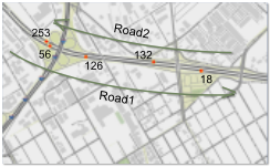
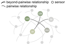
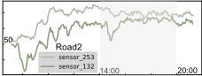
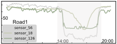
Figure 1: The illustration of complex relationships. As shown in (c), sensors on the same road tend to form a group and share common relationships and show similar characteristics. There may be various relationships connect with different numbers of sensors from multiple views. And one sensor may be influenced by many relationships. We demonstrate the complexity of relationships in (b).
modeling the relationships among variables properly is crucial for making precise predictions. Early traditional statistical methods, such as autoregressive integrated moving average (ARIMA) and Gaussian process model (GP), assume linear relationships among variables, which are not capable of handling many real-world data with complex relationships. These years have witnessed that many deep learning-based methods have been proposed to solve this problem. LSTNet [Lai et al., 2018] and TPA-LSTM [Shih et al., 2019] combine convolution neural networks (CNNs) and recurrent neural networks (RNNs) to extract local temporal patterns and long-term dependencies from MTS data, but they do not explicitly model the relationships. Recently, the success of graph neural networks (GNNs) in relational representing brings an innovative and promising way to MTS data modeling and leads to the birth of many graph-based methods. These methods treat MTS data as graph signals, whose nodes and edges represent time series variables and their relationships, respectively. Among them, some spatial-temporal graph neural networks (STGNNs) methods [Li et al., 2018; Yu et al., 2018] utilize pre-defined graph structures based on the distance between sensors on the road. STGNNs first apply graph convolution to solve traffic prediction problems. However, the graph structures are not available in all scenarios. Therefore, many data-driven strategies are proposed to learn graph structures from time series data and reduce the dependence on prior knowledge. MTGNN [Wu et al., 2020] first introduces the adaptive graph structure learning method and extracts uni-directional relationships between each pair of variables. ESG [Ye et al., 2022] puts effort into constructing evolutionary graphs to describe the dynamics of data. There are also some researchers working on improving the message passing mechanisms on graphs to further exploit these relationships [Zheng et al., 2020; Cao et al., 2020].
Although these methods benefit from learning relationships and achieve impressive success, we observe that they still lack comprehensive consideration in relational capturing and modeling. More specifically, there are two limitations to be addressed: 1) The existing methods treat MTS data as simple graphs and only capture pairwise relationships. However, the relationships may be more complex in practical scenarios. As shown in Figure 1, we visualize some time series data collected by sensors as well as the road map of PEMS-BAY dataset. The sensors on the same road attempt to show similar characteristics and form a group, thus sharing a common relationship. Considering that such sensor groups may have different numbers of sensors, we can discover complex relationships from multiple views. Different relationships may affect sensor groups of various sizes. It is difficult to comprehensively describe these complex relationships using only a simple graph. Accordingly, we demonstrate the potential hypergraph structure, whose edges connect with more than one node and are capable of modeling beyond-pairwise relationships. 2) The existing methods only focus on the existence of relationships, but not on other properties, like the categories. However, we notice that a time series variable may be influenced by many relationships and different relationships may have various impacts on time series variables. For instance, the rise and fall of the time series may be caused by influences from different relationships. It is helpful to promote precise behavior-modeling of time series variables if we can distinguish the potential impacts from different kinds of relationships.
Therefore, in this paper, we seek to learn complex relationships among time series variables from a more comprehensive perspective. By utilizing the methods in relational reasoning [Kipf et al., 2018; Xu et al., 2022] and hypergraph neural networks [Feng et al., 2019], we introduce the following approaches to tackle the aforementioned limitations. To capture multi-view complex relationships, we propose the time-specific Relational HyperGraph Constructor to adaptively infer a set of hypergraphs from MTS data. The time feature of data is considered to distinguish the relationships from different time periods. To exploit more properties of relationships, we introduce the Relational Modeling Module to learn the representations of relationships, which allows us to infer potential categories of relationships and thus distinguish their impacts. By integrating these components with the advanced temporal convolution module [Wu et al., 2020], we propose the MTS forecasting framework, namely ReMo, to comprehensively model the relationships and effectively improve the forecasting. Our contributions can be summarized as follows:
- We encourage considering the relationships among MTS data from multiple views and taking advantage of hypergraph in complex relationships representing, thus overcoming the limitation of existing graph-based methods in relational capturing.
- Unlike existing works that only focus on time series variables, we put efforts into fine-grained characterizing relationships. To this end, we propose to model the category-specific relationship explicitly through a novel hypergraph message passing strategy.
- Experimental results on real-world datasets show the effectiveness of our model as well as how the key components work to promote comprehensive relational modeling and improve the performance of forecasting.
2 Preliminaries
Definition 1 (Multivariate Time Series Forecasting). Multivariate Time Series with N variables can be denoted as X ∈ RT×N×C , where T is the number of timestamps, and C is the feature dimension which may vary in different scenarios. Xt ∈ RN×C indicates the values of all variables at timestamp t. MTS forecasting aims to exploit historical observed values with length P to predict future values with length F for all variables. It can be further divided into single-step forecasting and multi-step forecasting according to the desired prediction length. Given historical data with P timestamps Xt-P+1:t ∈ RP×N×C , single-step forecasting proposes to obtain future values Yt+F ∈ RN×C at fixed timestamp, while a sequence of future data Yt+1:t+F ∈ RF×N×C is needed for multi-step forecasting. To summarize, we aim to fit the mapping function F(·) from historical data to future data:
Definition 2 (Hypergraph). Different from edges in the simple graph, a hyperedge connects with two or more nodes and thus can indicate beyond-pairwise relationship. A hypergraph consisting of several nodes and hyperedges can be defined as G = (V, E), including a node set V and a hyperedge set E. The hypergraph G is usually denoted by a matrix H ∈ R|V|×|E| , whose elements are defined as:
where v ∈ V, e ∈ E and v ∈ e if the hyperedge e connect with node v.
3 Methodology
This section describes our proposed ReMo in details.
3.1 Overview
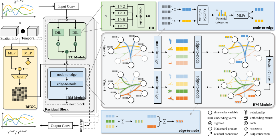
Here we introduce the overall architecture of the proposed model. As shown in Figure 2, ReMo consists of an input processor, a Relational HyperGraph Constructor (RHGC), some stacked Residual Blocks, and an output processor. To distinguish the complex relationships among time series variables in different time periods, the Relational HyperGraph Constructor infers a set of hypergraphs to represent multi-view relationships. Based on the hypergraphs, Residual Blocks comprehensively extract temporal features from time series variables and model the relationships among them with two modules, namely Temporal Convolution Module (TC Module) and Relational Modeling Module (RM Module). Specifically, the TC Module extracts temporal patterns with different ranges through two dilated inception layers. RMModule further infers the potential categories of relationships and performs hypergraph message passing to obtain nodes and hyperedges representations. By adding residual connections and skip connections, we stack the Residual Blocks and generate the final output. The input processor and the output processor are responsible for handling input data and output data from skip connections, respectively. For more details, these components will be stated elaborately in the rest of this section.
3.2 Relational Hypergraph Constructor
Due to the pairwise connectivity of its edges, a simple graph is often difficult to reflect complete relationships among time series variables in practical scenarios. Therefore, we seek a more flexible way, hypergraph, to capture complex relationships. Specifically, we treat time series variables as nodes and use a set of hypergraphs whose edges contain different numbers of nodes to represent multi-view relationships. Besides, we find that relationships may evolve over time, which inspires us to take the temporal features of data into account. Considering these two aspects, this module aims to infer multi-view hypergraphs from MTS data adaptively. Formally, given the set of N time series variables V = {V1, V2, ..., VN}, we aim to infer a set of hypergraphs G = {G p1 , G p2 , ..., G pn } to describe relationships from multiple views. For each view pi, let G pi = (V, E pi ) or the corresponding adjacency matrix Hpi denote the hypergraph and E pi = {epi 1 , epi 2 , ..., epiM } be the set of hyperedges, where M is the number of hyperedges. Each hyperedge contains pi nodes.
To construct multi-view hypergraphs, we adopt a nodewise similarity-based approach to adaptively learn G from data. Firstly, we initialize the node embeddings as Es ∈ RN×D1 . To fully exploit the temporal information, we then encode the time-in-day feature of nodes as Et ∈ RN×D2 . For any view pi, we extract corresponding Hpi by:
where both f1(·) and f2(·) are implemented by MLPs, and Hpi ∈ RM×N indicates the hypergraph for view pi and will be optimized during training stage. All obtained hypergraphs are fed into RMModule for further relational modeling.
3.3 Relational ModelingModule
Given the graph structures, most existing works treat edges only as bridges for aggregating the features of nodes, thus ignoring the other characteristics of the edges apart from their existence. However, relationships among time series variables may act in very different ways, which leads to various impacts on time series variables and cause complex behaviors. Therefore, fine-grained relationships modeling will allow us to exploit more valuable information and model the behavior of time series variables more precisely.
In this module, we take a step forward and ask: what types of relationships may exist among MTS data and how do they affect relevant variables? To answer this, we improve a hypergraph message passing strategy to learn the representations of both nodes and hyperedges from a more comprehensive perspective. Specifically, we execute message passing through two stages, namely node-to-edge stage and edge-tonode stage, to characterize relationships and extract valuable information, see Figure 2. In node-to-edge stage, we obtain the features of each hyperedge by aggregating the features of nodes it connects with. Then we infer the potential categories of hyperedges and define category-specific MLPs to further encode the features of hyperedges. In edge-to-node stage, nodes embeddings are updated by aggregating the features of relevant hyperedges to fuse the impacts of various relationships.
Node-to-edge. Given adjacency matrix H and nodes embeddings E(0) n , node-to-edge stage aims to obtain hyperedges embeddings E(1) e . Firstly, we apply convolution operation on hypergraph to aggregate the features of nodes and generate initial hyperedges embeddings E(0) e :
where the learnable parameter Θn is applied over nodes embeddings to extract important features and indicates the contribution of the nodes to the hyperedges. Secondly, we infer the potential categories from hyperedges embeddings through Gumbel Softmax following [Maddison et al., 2017; Jang et al., 2017]:
where C ∈ RM×K is the concrete distribution used as a continuous approximation of the discrete categorical distribution, and ∑k cm,k = 1. g is a vector whose elements are i.i.d. samples drawn from a Gumble(0, 1) distribution and τ is a temperature parameter that controls the smoothness of the samples. fc(·) is also implemented by MLPs. Then we encode the categorical features of hyperedges and obtain the final embeddings of hyperedges:
where f (k) e (·) is the category-specific mapping function implemented by MLPs. We define different fe(·) to encode hyperedges with different categories and distinguish various impacts of relationships.
Edge-to-node. The behavior of nodes is usually influenced by multiple relationships. In the edge-to-node stage, we find all relevant relationships for each time series variable and fuse the complex impacts. Formally, given learned hyperedges embeddings, node embeddings are updated by executing the hypergraph convolution again:
where Θe is the parameter applied over edges to filter the information during feature aggregation. Thus far, we obtain the final representation of the nodes by comprehensively relational modeling. It is worth mentioning that the node-to-edge and edge-to-node stages can be executed for multiple iterations if necessary. RMModule updates the node features of multiple hypergraphs in parallel, and finally fuses information from multiple views through a convolution layer with a kernel of size 1 × nview and a dilation factor of dfuse, where nview and dfuse indicate the number of views and the dimension of node embeddings, respectively.
3.4 Temporal ConvolutionModule
Capturing intra-variable long-term dependency and discovering valuable temporal patterns are also crucial for understanding the behavior of time series and making better predictions. However, it is challenging to both discover temporal patterns with different ranges and handle long sequences. Here we introduce the Dilated Inception Layer (DIL) proposed by [Wu et al., 2020] to address these problems.
DIL applies dilated convolution to get wider receptive fields with less computation cost. It makes the receptive field expand exponentially with the increase of the layers by using the dilation factor. Given input sequence z ∈ RT and 1D convolution filter kernel f1×k ∈ Rk with size k, the dilated convolution is defined as:
where d is the dilation factor. To discover patterns with various ranges, DIL utilizes multi-size filters and performs multiple convolutions in parallel on the input sequence. Finally, we concatenate the outputs of DIL to comprehensively exploit the features of different patterns:
The temporal convolution module consists of two DILs, which are followed by a tangent hyperbolic activation function and a sigmoid activation function, respectively. These activation functions work as a gate to control the amount of information that should pass to the next module:
3.5 Input &Output Processor
Input processor implemented by a standard convolution layer with 1 × 1 filter takes raw data as inputs and expands the channel dimension. Output processor consists of three standard convolution layers with 1 × 1 filters and projects the hidden features to a fixed dimension according to the prediction length and target number of channels. Specifically, it first takes the output sequence from skip connections as inputs and transforms the length dimension into target prediction length, then projects the hidden features to fixed channel dimension according to the demands of different tasks.
| Model | NYC-Bike | PEMS-BAY | PEMSD8 | ||||||
|---|---|---|---|---|---|---|---|---|---|
| MAE↓ | RMSE↓ | MAPE↓ | MAE↓ | RMSE↓ | MAPE↓ | MAE↓ | RMSE↓ | MAPE↓ | |
| DCRNN | 1.90 | 3.23 | - | 1.75 | 4.07 | 4.21% | 16.82 | 26.36 | 10.92% |
| STGCN | 2.21 | 3.78 | - | 2.50 | 4.93 | 4.02% | 17.50 | 27.09 | 11.29% |
| GraphWaveNet | 2.45 | 4.37 | 60.93% | 2.17 | 4.61 | 5.31% | 22.19 | 33.15 | 15.01% |
| MTGNN | 1.82 | 3.30 | 58.44% | 1.72 | 3.71 | 3.94% | 17.01 | 26.50 | 11.18% |
| AGCRN | 1.92 | 3.60 | 60.58% | 1.81 | 4.11 | 4.15% | 16.71 | 26.50 | 10.64% |
| ESG | 1.77 | 3.17 | 59.40% | 1.89 | 4.07 | 4.66% | 18.17 | 27.40 | 17.90% |
| Ours | 1.66 | 2.86 | 57.74% | 1.66 | 3.65 | 3.81% | 16.36 | 25.54 | 10.85% |
| Dataset | Nodes | Samples | Interval | Task |
|---|---|---|---|---|
| Solar-Energy | 137 | 52560 | 10 min | Single-step |
| Electricity | 321 | 26304 | 1 hour | Single-step |
| Wind | 28 | 10957 | 1 day | Single-step |
| Exchange-Rate | 8 | 7588 | 1 day | Single-step |
| NYC-Bike | 250 | 4368 | 30 min | Multi-step |
| PEMS-BAY | 325 | 52116 | 5 min | Multi-step |
| PEMSD8 | 170 | 17833 | 5 min | Multi-step |
4 Experiments
In this section, we extensively evaluate the proposed ReMo on seven commonly used MTS datasets. Then we further demonstrate how the modules of ReMo contribute to the performance.
4.1 Experimental Setup
Datasets. Four MTS benchmark datasets and three realworld traffic datasets are selected for different tasks, respectively. We summarize the statistical information of these datasets in Table 2.
Baselines. Six popular baselines are selected for single-step forecasting containing Auto-Regressive(AR), GP [Roberts et al., 2013], LSTNet [Lai et al., 2018], TPA-LSTM [Shih et al., 2019], MTGNN [Wu et al., 2020], ESG [Ye et al., 2022]. For multi-step forecasting, we also select six advanced graph-based baselines, including DCRNN [Li et al., 2018], STGCN [Yu et al., 2018], Graph WaveNet [Wu et al., 2019], MTGNN [Wu et al., 2020], AGCRN [Bai et al., 2020], and ESG [Ye et al., 2022].
Evaluation Metrics. For single-step forecasting, we adopt Root Relative Squared Error (RSE) and Empirical Correlation Coefficient (CORR) to evaluate the performances of all baselines. Three commonly used metrics are selected for multi-step forecasting, including Mean Absolute Error
(MAE), Root Mean Squared Error (RMSE), and Mean Absolute Percentage Error (MAPE).
Implementation Details. The proposed model is implemented with Pytorch 1.12.1 on an NVIDIA GeForce RTX 3090 GPU and trained by the Adam optimizer with gradient clip 5. We set the length of historical data P to 168 and prediction length F to 1 for single-step forecasting. In the multi-step case, we have P = F = 12.
4.2 Main Results
Table 1 and Table 3 summarize the overall experimental results on multi-step and single-step forecasting.
Multi-step forecasting. For the multi-step forecasting task, we validate the performance of our ReMo and other graphbased methods by comparing the average values of MAE, RMSE, MAPE metrics on all 12 horizons. The complex spatial-temporal characteristics of traffic data make it difficult to comprehensively capture and model the relationships. Therefore, methods focused on different aspects of relational modeling may achieve different results. In general, ReMo achieves state-of-the-art results on all datasets. It lowers MAE by 6.21% and RMSE by 8.83% on NYC-Bike and also makes slight improvements on other datasets. To illustrate the results, we make the following analysis: 1) DCRNN and STGCN are limited due to heavy dependence on pre-defined graph structures and the neglect of the feature in the raw data. 2) The adaptive methods, like MTGNN, Graph WaveNet, and AGCRN, extract the relationships from time series data and slightly improve the performance. 3) ESG further simulates the evolution of relationships and is more suitable for systems with complex dynamics. However, ReMo captures relationships from multiple views and distinguishes the impacts of different relationships by inferring their potential categories, which allows it to model the behavior of variables more comprehensively.
Single-step forecasting. For the single-step task, we compare ReMo with other classical MTS forecasting methods. Specifically, the performance of models on horizon 3, 6, 12, and 24 of all datasets are compared. Table 3 shows the detailed results. In general, ReMo shows strong competitiveness. It outperforms baselines on four horizons on ExchangeRate dataset and on horizon 12 and 24 on Solar-Energy dataset. However, the performance has not been improved on the other two datasets. This is possibly because of the characteristics of the datasets. Electricity collects the electricity consumption of different households. Wind dataset demonstrates the power of different windmills in the same area. The common characteristic of these two datasets is that time series variables demonstrate greater independence, which may lead to weak relationships among them and overly detailed relational modeling is too much in these cases.
| Model | Dataset Horizon | Solar-Energy | Electricity | Exchange-Rate | Wind | ||||||||||||
|---|---|---|---|---|---|---|---|---|---|---|---|---|---|---|---|---|---|
| 3 | 6 | 12 | 24 | 3 | 6 | 12 | 24 | 3 | 6 | 12 | 24 | 3 | 6 | 12 | 24 | ||
| AR | RSE↓ CORR↑ | 0.2345 0.9710 | 0.3790 0.9263 | 0.5911 0.8107 | 0.8699 0.5314 | 0.0995 0.8845 | 0.1035 0.8632 | 0.1050 0.8591 | 0.1054 0.8595 | 0.0228 0.9734 | 0.0279 0.9656 | 0.0353 0.9526 | 0.0445 0.9357 | 0.7161 0.6459 | 0.7572 0.6046 | 0.8076 0.5560 | 0.9371 0.4633 |
| GP | RSE↓ CORR↑ | 0.2259 0.9751 | 0.3286 0.9448 | 0.5200 0.8518 | 0.7973 0.5971 | 0.1500 0.8670 | 0.1907 0.8334 | 0.1621 0.8394 | 0.1273 0.8818 | 0.0239 0.8713 | 0.0272 0.8193 | 0.0394 0.8484 | 0.0580 0.8278 | 0.6689 0.6964 | 0.6761 0.6877 | 0.6772 0.6846 | 0.6819 0.6781 |
| LSTNet | RSE↓ CORR↑ | 0.1843 0.9843 | 0.2559 0.9690 | 0.3254 0.9467 | 0.4643 0.8870 | 0.0864 0.9283 | 0.0931 0.9135 | 0.1007 0.9077 | 0.1007 0.9119 | 0.0226 0.9735 | 0.0280 0.9658 | 0.0356 0.9511 | 0.0449 0.9354 | 0.6079 0.7436 | 0.6262 0.7275 | 0.6279 0.7249 | 0.6257 0.7284 |
| TPA-LSTM | RSE↓ CORR↑ | 0.1803 0.9850 | 0.2347 0.9742 | 0.3234 0.9487 | 0.4389 0.9081 | 0.0823 0.9439 | 0.0916 0.9337 | 0.0964 0.9250 | 0.1006 0.9133 | 0.0174 0.9790 | 0.0241 0.9709 | 0.0341 0.9564 | 0.0444 0.9381 | 0.6093 0.7433 | 0.6292 0.7240 | 0.6290 0.7235 | 0.6335 0.7202 |
| MTGNN | RSE↓ CORR↑ | 0.1815 0.9846 | 0.2381 0.9723 | 0.3139 0.9500 | 0.4287 0.9007 | 0.0751 0.9463 | 0.0839 0.9348 | 0.0913 0.9257 | 0.0965 0.9209 | 0.0252 0.9737 | 0.0298 0.9663 | 0.0367 0.9529 | 0.0462 0.9331 | 0.6204 0.7337 | 0.6346 0.7209 | 0.6363 0.7164 | 0.6426 0.7134 |
| ESG | RSE↓ CORR↑ | 0.1814 0.9845 | 0.2370 0.9721 | 0.3118 0.9494 | 0.4287 0.9019 | 0.0754 0.9423 | 0.0854 0.9312 | 0.0914 0.9265 | 0.1000 0.9194 | 0.0238 0.9771 | 0.0297 0.9686 | 0.0368 0.9564 | 0.0497 0.9361 | 0.6146 0.7374 | 0.6247 0.7297 | 0.6230 0.7281 | 0.6349 0.7194 |
| Ours | RSE↓ CORR↑ | 0.1877 0.9834 | 0.2419 0.9713 | 0.3112 0.9507 | 0.4244 0.9027 | 0.0779 0.9381 | 0.0879 0.9227 | 0.0949 0.9167 | 0.1011 0.9058 | 0.0173 0.9753 | 0.0240 0.9680 | 0.0340 0.9565 | 0.0443 0.9373 | 0.6191 0.7330 | 0.6311 0.7211 | 0.6310 0.7214 | 0.6391 0.7177 |
4.3 Ablation Study
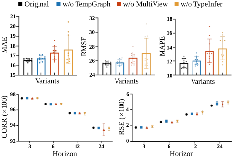
To better understand how the key components contribute to ReMo, We conduct ablation studies on PEMSD8 and Exchange-Rate. By disabling different components, we can obtain some variants of ReMo. For clarity, we name these variants as follows:
- w/o TempGraph: Ignoring the time-in-day features when constructing multiple hypergraphs. The multiview hypergraphs construction is based on the spatial features only.
- w/o MultiView: Capturing and modeling relationships from one specific view. Specifically, the views are set differently according to the number of time series vari-
- ables on different datasets. For PEMSD8, a view is a natural number in the range of 170. For Exchange-Rate, the range is 8.
- w/o EdgeType: Skipping the potential categories inference of hyperedges during node-to-edge stage. In this case, hyperedges embedding obtained by hypergraph convolution operation are fed into the edge-tonode stage directly.
- Original: Standing for proposed ReMo with all key components enabled.
Applying the original ReMo and its variants, we repeat each experiment 10 times and report the average values of metrics for all horizons in Figure 3. In particular, for capturing single-view relationships, we obtain the value of the view by randomly sampling from its range of potential values. As can be seen from Figure 3, the experimental results validate the effectiveness of these components to a certain extent.
The original ReMo outperforms other variants by a large margin on PEMSD8 dataset. It lowers MAE by 3.78%, RMSE by 2.79%, and MAPE by 10.09% on average and brings smaller standard deviations to the results. Constructing hypergraphs without considering the temporal features still reaches competitive results, which means adaptive graph structure learning methods work for MTS forecasting. While only capturing single-view relationships and removing the potential categories inference when characterizing relationships reach worse results, which indicates incomprehensive relationships modeling cannot fully exploit valuable information. However, the improvement on Exchange-Rate Dataset is relatively small. It slightly improves the RSE and has few contributions to raising the CORR. The results are consistent with our intuition. This is because Exchange-Rate dataset has a smaller size and the exchange rate usually changes with irregular rules in the real-world. Therefore, less information can be exploited to both capture and model relationships, which may lead to over-modeling for our model. Overall, considering the multiple views and temporal features of relationships brings more comprehensive capturing and modeling of relationships. The effort on inferring the potential categories of relationships allows us to distinguish the impacts they have on various variables. The key components of ReMo work together and promote more precise behavior-modeling of time series variables.
4.4 Visualization of Complex Relationships
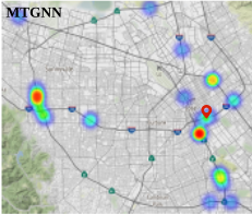
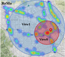
To further demonstrate the complexity of relationships, we visualize the relationships that MTGNN and our ReMo capture in Figure 4. Specifically, we show the correlation between 233th sensor and other sensors on PEMS-BAY dataset in the form of heatmaps. It is worth mentioning that the goal of relationship capturing is to find valuable information from other sensors to promote precise prediction for the specific sensor, but not to construct the ground truth graph structure. In this case, MTGNN finds 20 related sensors although their distances to 233th sensor are very far. However, considering relationships from one specific view may lead to missing information. Therefore we encourage capturing the relationships from multiple views. As shown in Figure 4, we demonstrate the relationships from two views ReMo captures. In view0, ReMo focuses on the nearby sensors more. The remote sensors are taken into account in view1. For traffic prediction problems, sensors are more directly affected by their immediate neighbors and may have delayed effects from remote sensors. Capturing different relationships frommultiple views is helpful to capture comprehensive impacts from relationships and promote fine-grained modeling of the behaviors of time series variables.
5 RelatedWork
Time series forecasting. Time series forecasting has been extensively studied for a long time [Lim and Zohren, 2021]. Here we mainly focus on the advanced deep learning methods for MTS forecasting. LSTNet [Lai et al., 2018] and TPA-LSTM [Shih et al., 2019] are the earliest deep learning methods applied to MTS forecasting. They both combine convolution neural networks (CNNs) and recurrent neural networks (RNNs) to capture temporal patterns and intravariable dependencies, respectively. However, CNNs are not capable of modeling fine-grained dependencies between time series variables due to the aggregation operation. Recently, some graph-based methods achieve significant success in MTS forecasting. Spatial-temporal graph neural networks (STGNNs) are proposed to solve traffic prediction problems [Li et al., 2018; Yu et al., 2018]. This kind of method utilizes pre-defined graph structures (e.g. road sensor location map) to describe the relationships between time series and leverage graph convolution to capture the impacts of relationships. Although they have significantly improved the forecasting performance, they still lack generality due to excessive dependence on the external graph structure, which is usually unknown in many scenarios. To solve this problem, Graph WaveNet [Wu et al., 2019] and MTGNN [Wu et al., 2020] propose data-driven methods to adaptively extract graph structure from MTS data without any prior knowledge. ESG [Ye et al., 2022] further extend them to model the evolution of relationships and further simulates the dynamics of MTS data. Z-GCNETs [Chen et al., 2021] and RGSL [Yu et al., 2022] utilize both explicit and implicit relationships to improve the graph structures. However, they only model pairwise relationships.
Hypergraph Neural Networks. Hypergraph learning is first introduced in [Zhou et al., 2006] for modeling complex relationships among objects and has been extensively studied for the past few years. HGNN [Feng et al., 2019] designs a node-hyperedge-node message propagation strategy to learn data representation on hypergraphs. HyperGCN [Yadati et al., 2019] proposed a new method of training a GCN on hypergraphs based on spectral theory. A hyperedge-node attention learning module is introduced to identify different importance of nodes in the same hyperedge, thus generating more discriminative node embeddings [Bai et al., 2021].
Relational reasoning. Some previous works attempt to model the relationships between objects in complex systems. NRI [Kipf et al., 2018] infers an explicit static relational graph and learns the dynamics of latent variables via GNNs. IMMA [Sun et al., 2022] uses multiple latent graphs and attention to describe different types and strengths of relationships. A multi-scale approach is proposed to comprehensively model the group interaction relationships in multiagent systems and improve the accuracy of trajectory predictions [Xu et al., 2022].
6 Conclusion
We find that when modeling multivariate time series, in addition to pairwise relationships, capturing beyond-pairwise relationships from multiple views and distinguishing their potential categories are also crucial for improving forecasting performance. Therefore, we introduce a novel approach to promote fine-grained relational modeling. Extensive experiments demonstrate the effectiveness of our model. In particular, we achieve this by learning the multi-view hypergraphs to capture complex relationships more comprehensively and further inferring the potential categories of these relationships to distinguish their impacts on time series variables, thus promoting precise behavior-modeling of time series variables. It is an interesting attempt and provides a valuable perspective to demystify the relationships among multivariate time series data, which may lead to a breakthrough in interpretability.
Acknowledgments
This work was supported in part by the National Natural Science Foundation of China under Grants (62171057, 62101064, 62201072, 62071067, 62001054), in part by the Ministry of Education and China Mobile Joint Fund (MCM20200202), Beijing University of Posts and Telecommunications-China Mobile Research Institute Joint Innovation Center.
Contribution Statement
Jinming Wu and Qi Qi contributed equally to this work.
@inproceedings{ijcai2023p491,
  title     = {Not Only Pairwise Relationships: Fine-Grained Relational Modeling for Multivariate Time Series Forecasting},
  author    = {Wu, Jinming and Qi, Qi and Wang, Jingyu and Sun, Haifeng and Wu, Zhikang and Zhuang, Zirui and Liao, Jianxin},
  booktitle = {Proceedings of the Thirty-Second International Joint Conference on
               Artificial Intelligence, {IJCAI-23}},
  publisher = {International Joint Conferences on Artificial Intelligence Organization},
  editor    = {Edith Elkind},
  pages     = {4416--4423},
  year      = {2023},
  month     = {8},
  note      = {Main Track},
  doi       = {10.24963/ijcai.2023/491},
  url       = {https://doi.org/10.24963/ijcai.2023/491},
}
TY - CPAPER TI - Not Only Pairwise Relationships: Fine-Grained Relational Modeling for Multivariate Time Series Forecasting AU - Wu, Jinming AU - Qi, Qi AU - Wang, Jingyu AU - Sun, Haifeng AU - Wu, Zhikang AU - Zhuang, Zirui AU - Liao, Jianxin T2 - Proceedings of the Thirty-Second International Joint Conference on Artificial Intelligence, IJCAI-23 PB - International Joint Conferences on Artificial Intelligence Organization PY - 2023 SP - 4416 EP - 4423 DO - 10.24963/ijcai.2023/491 UR - https://doi.org/10.24963/ijcai.2023/491 ER -Copied
Machine-readable versions of this paper, for tools and AI agents:





