
LGPConv: Learnable Gaussian Perturbation Convolution for Lightweight Pansharpening
Proceedings of the Thirty-Second International Joint Conference on Artificial Intelligence. Main Track. Pages 4647-4655.
https://doi.org/10.24963/ijcai.2023/517
Keywords
- Computer Vision: CV: Machine learning for vision
- Machine Learning: ML: Convolutional networks
- Machine Learning: ML: Applications
Abstract
Pansharpening is a crucial and challenging task that aims to obtain a high spatial resolution image by merging a multispectral (MS) image and a panchromatic (PAN) image. Current methods use CNNs with standard convolution, but we've observed strong correlation among channel dimensions in the kernel, leading to computational burden and redundancy. To address this, we propose Learnable Gaussian Perturbation Convolution (LGPConv), surpassing standard convolution. LGPConv leverages two properties of standard convolution kernels: 1) correlations within channels, learning a premier kernel as a base to reduce parameters and training difficulties caused by redundancy; 2) introducing Gaussian noise perturbations to simulate randomness and enhance nonlinear representation within channels. We incorporate LGPConv into a well-designed pansharpening network and demonstrate its superiority through extensive experiments, achieving state-of-the-art performance with minimal parameters (27K). Code is available on the GitHub page of the authors.
- [Aiazzi et al., 2006] Bruno Aiazzi, L Alparone, Stefano Baronti, Andrea Garzelli, and Massimo Selva. Mtf- tailored multiscale fusion of high-resolution ms and pan imagery. Photogrammetric Engineering & Remote Sensing, 72(5):591-596, 2006.
- [Cao et al., 2022] Xiangyong Cao, Xueyang Fu, Danfeng Hong, Zongben Xu, and Deyu Meng. Pancsc-net: A model- driven deep unfolding method for pansharpening. IEEE Transactions on Geoscience and Remote Sensing, 60:1-13, 2022.
- [Deng et al., 2021] Liang-Jian Deng, Gemine Vivone, Cheng Jin, and Jocelyn Chanussot. Detail injection-based deep convolutional neural networks for pansharpening. IEEE Transactions on Geoscience and Remote Sensing, 59(8):6995-7010, 2021.
- [Fu et al., 2019] Xueyang Fu, Zihuang Lin, Yue Huang, and Xinghao Ding. A variational pan-sharpening with local gradient constraints. In CVPR, pages 10265-10274, 2019.
- [Fu et al., 2020] Xueyang Fu, Wu Wang, Yue Huang, Xing- hao Ding, and John Paisley. Deep multiscale detail net- works for multiband spectral image sharpening. IEEE Transactions on Neural Networks and Learning Systems, 32(5):2090-2104, 2020.
- [Garzelli et al., 2007] Andrea Garzelli, Filippo Nencini, and Luca Capobianco. Optimal mmse pan sharpening of very high resolution multispectral images. IEEE Transactions on Geoscience and Remote Sensing, 46(1):228-236, 2007.
- [Guo et al., 2020a] Penghao Guo, Peixian Zhuang, and Yecai Guo. Bayesian pan-sharpening with multiorder gradient- based deep network constraints. IEEE Journal of Selected Topics in Applied Earth Observations and Remote Sensing, 13:950-962, 2020.
- [Guo et al., 2020b] Penghao Guo, Peixian Zhuang, and Yecai Guo. Bayesian pan-sharpening with multiorder gradient- based deep network constraints. IEEE Journal of Selected Topics in Applied Earth Observations and Remote Sensing, 13:950-962, 2020.
- [Haase and Amthor, 2020] Daniel Haase and Manuel Amthor. Rethinking depthwise separable convolutions: How intra- kernel correlations lead to improved mobilenets. In IEEE Conf. Comput. Vis. Pattern Recog. (CVPR), pages 14600- 14609, 2020.
- [He et al., 2019] Lin He, Yizhou Rao, Jun Li, Jocelyn Chanus- sot, Antonio Plaza, Jiawei Zhu, and Bo Li. Pansharpening via detail injection based convolutional neural networks. IEEE Journal of Selected Topics in Applied Earth Observa- tions and Remote Sensing, 12(4):1188-1204, 2019.
- [Hein and Andriushchenko, 2017] Matthias Hein and Maksym Andriushchenko. Formal guarantees on the robustness of a classifier against adversarial manipulation. In I. Guyon, U. Von Luxburg, S. Bengio, H. Wallach, R. Fergus, S. Vishwanathan, and R. Garnett, editors, Adv. Neural Inform. Process. Syst. (NIPS), volume 30, 2017.
- [Howard et al., 2017] Andrew G Howard, Menglong Zhu, Bo Chen, Dmitry Kalenichenko, Weijun Wang, Tobias Weyand, Marco Andreetto, and Hartwig Adam. Mobilenets: Efficient convolutional neural networks for mobile vision applications. arXiv preprint arXiv:1704.04861, 2017.
- [Jin et al., 2022a] Cheng Jin, Liang-Jian Deng, Ting-Zhu Huang, and Gemine Vivone. Laplacian pyramid networks: A new approach for multispectral pansharpening. Informa- tion Fusion, 78:158-170, 2022.
- [Jin et al., 2022b] Zi-Rong Jin, Tian-Jing Zhang, Tai-Xiang Jiang, Gemine Vivone, and Liang-Jian Deng. Lagconv: Local-context adaptive convolution kernels with global harmonic bias for pansharpening. AAAI Conference on Artificial Intelligence (AAAI), 36(1):1113-1121, 2022.
- [Liu et al., 2018] Xuanqing Liu, Minhao Cheng, Huan Zhang, and Cho-Jui Hsieh. Towards robust neural networks via random self-ensemble. In ECCV, pages 369-385, 2018.
- [Masi et al., 2016a] Giuseppe Masi, Davide Cozzolino, Luisa Verdoliva, and Giuseppe Scarpa. Pansharpening by convo- lutional neural networks. Remote Sensing, 8(7):594, 2016.
- [Masi et al., 2016b] Giuseppe Masi, Davide Cozzolino, Luisa Verdoliva, and Giuseppe Scarpa. Pansharpening by convo- lutional neural networks. Remote Sensing, 8(7):594, 2016.
- [Meyer, 2000] Carl Meyer. Matrix Analysis and Applied Lin- ear Algebra Book and Solutions Manual. 01 2000.
- [T.-J. Zhang and Vivone, 2022] T.-Z. Huang J. Chanussot T.- J. Zhang, L.-J. Deng and G. Vivone. A triple-double convo- lutional neural network for panchromatic sharpening. IEEE Transactions on Neural Networks and Learning Systems, 2022.
- [Vivone et al., 2020] Gemine Vivone, Mauro Dalla Mura, An- drea Garzelli, Rocco Restaino, Giuseppe Scarpa, Magnus O Ulfarsson, Luciano Alparone, and Jocelyn Chanussot. A new benchmark based on recent advances in multispectral pansharpening: Revisiting pansharpening with classical and emerging pansharpening methods. IEEE Geoscience and Remote Sensing Magazine, 9(1):53-81, 2020.
- [Weng et al., 2018] Tsui-Wei Weng, Huan Zhang, Pin-Yu Chen, Jinfeng Yi, Dong Su, Yupeng Gao, Cho-Jui Hsieh, and Luca Daniel. Evaluating the robustness of neural net- works: An extreme value theory approach, 2018.
- [Yan et al., 2022a] Keyu Yan, Man Zhou, Jie Huang, Feng Zhao, Chengjun Xie, Chongyi Li, and Danfeng Hong. Panchromatic and multispectral image fusion via alter- nating reverse filtering network. In Alice H. Oh, Alekh Agarwal, Danielle Belgrave, and Kyunghyun Cho, editors, Advances in Neural Information Processing Systems, 2022.
- [Yan et al., 2022b] Yinsong Yan, Junmin Liu, Shuang Xu, Yicheng Wang, and Xiangyong Cao. Md³net: Integrating model-driven and data-driven approaches for pansharpen- ing. IEEE Transactions on Geoscience and Remote Sensing, 60:1-16, 2022.
- [Yang et al., 2017] Junfeng Yang, Xueyang Fu, Yuwen Hu, Yue Huang, Xinghao Ding, and John Paisley. Pannet: A deep network architecture for pan-sharpening. In Int. Conf. Comput. Vis. (ICCV), pages 5449-5457, 2017.
- [Yang et al., 2020] Yong Yang, Chenxu Wan, Shuying Huang, Hangyuan Lu, and Weiguo Wan. Pansharpening based on low-rank fuzzy fusion and detail supplement. IEEE Journal of Selected Topics in Applied Earth Observations and Remote Sensing, 13:5466-5479, 2020.
- [Yuan et al., 2018] Qiangqiang Yuan, Yancong Wei, Xi- angchao Meng, Huanfeng Shen, and Liangpei Zhang. A multiscale and multidepth convolutional neural network for remote sensing imagery pan-sharpening. IEEE Journal of Selected Topics in Applied Earth Observations and Remote Sensing, 11(3):978-989, 2018.
- [Zhang et al., 2019] Yongjun Zhang, Chi Liu, Mingwei Sun, and Yangjun Ou. Pan-sharpening using an efficient bidirec- tional pyramid network. IEEE Transactions on Geoscience and Remote Sensing, 57(8):5549-5563, 2019.
- [Zhou et al., 2022] Man Zhou, Jie Huang, Keyu Yan, Hu Yu, Xueyang Fu, Aiping Liu, Xian Wei, and Feng Zhao. Spatial- frequency domain information integration fornbsp;pan- sharpening. page 274-291, Berlin, Heidelberg, 2022. Springer-Verlag.
- [Zhuang et al., 2019] Peixian Zhuang, Qingshan Liu, and Xinghao Ding. Pan-ggf: A probabilistic method for pan- sharpening with gradient domain guided image filtering. Signal Processing, 156:177-190, 2019.
References were extracted automatically from the PDF and may contain errors.
Full text extracted automatically from the PDF; figures, tables and equations may differ. The PDF is the version of record.
1 Introduction
With the rapid development of satellite sensors, remote sensing images have become widely used in many fields, i.e., classification, super-resolution, pansharpening, and so on. However, because of the physical limitations of remote sensing imaging devices, images with high spatial and spectral resolutions are hard to achieve by a single sensor. The most typical solution is to make a trade-off between the spatial and spectral resolutions. Therefore, pansharpening, which aims at fusing a low resolution multispectral (LR-MS) image and panchromatic (PAN) data and yielding a high spatial resolution MS image (HR-MS), has become a fundamental task in remote sensing image processing.
This work is supported by NSFC (12271083) and Natural Science Foundation of Sichuan Province (2022NSFSC0501).
* The corresponding author: Liang-Jian Deng
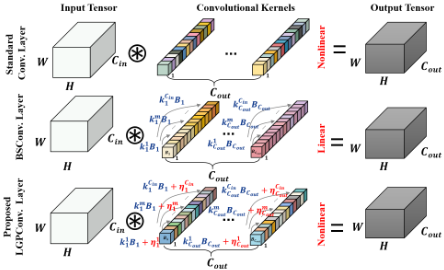
Many research efforts have been donated to pansharpening, which can be divided into four groups, i.e., component substitution (CS), multiresolution analysis (MRA), variational optimization (VO), and deep learning (DL) based methods. A detailed review can be found in [Vivone et al.2020]. However, the first three methods restrict performance and optimization. With the advancements of hardware in image processing applications, DL-based methods, particularly convolution neural networks (CNNs)-based techniques, are emerging lines of pansharpening [Guo et al.2020a,Yang et al.2020, T.-J. Zhang and Vivone2022, Jin et al.2022b, Zhou et al.2022,Yan et al.2022a]. However, these DL-based methods often acquire a large number of parameters and suffer from high computational costs and low efficiency.
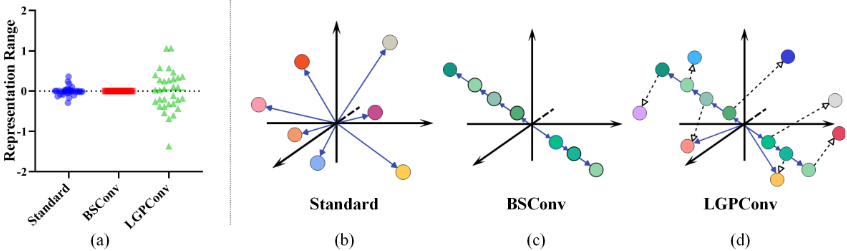
CNNs have achieved state-of-the-art (SOTA) in many image restoration tasks such as super-resolution, denoising, and pansharpening. The standard convolution focuses on feature extraction and correlation between spatial and channel dimensions. However, the number of parameters of existing convolution kernels depends on the number of channels of the target feature map. The correlation among channels often makes the convolution kernels redundant. In order to improve the performance and reduce redundancy, many previous attempts have tried to address these issues and have obtained relatively good performances. MobileNets [Howard et al.2017] proposed a lightweight structure called a depthwise separable convolution (DSC) module. The DSC module factorizes a standard convolution into a depthwise convolution and a pointwise convolution. In 2020, Hasse et al. [Haase and Amthor2020] exploited high redundancy in DSC by visualizing the learned filter kernels, which showed intra-kernel correlations along the depth axis of convolution kernels. Thus, they proposed blueprint separable convolutions (BSConv) with a "blueprint" convolution kernel to generate the whole one and cut down the parameters successfully. However, BSConv has limited representation capability due to its ease of transformation (see Fig. 1 and Fig. 3). For more reviews, please see related works. The main contributions of this paper can be summarized as follows:
- We propose a novel generation of convolution kernels based on channel-wise linear transformation of kernels and noise perturbation bias, namely LGPConv, which uses randomness of noise to achieve kernel nonlinearity. It provides high efficiency for feature representation and facilitates network training with small parameters.
- Using linear algebra, we conduct an in-depth analysis of the unnecessary redundancy caused by the original kernel generation and demonstrate the latent correlation and difference among convolution kernel channels. In addition, we theoretically prove LGPConv's convergence and explain its implementation in detail.
- Comprehensive analysis on pansharpening performance of our method is conducted through ablation studies, qualitative and quantitative results. Also, to the best of our knowledge, the proposed method can achieve SOTA performance with a small parameter scale (only 27K).
2 RelatedWorks andMotivations
2.1 CNNs for Pansharpening
As one of the DL-based methods for pansharpening, CNNs have been widely applied in this area by virtue of their powerful nonlinear fitting capabilities. In 2016, Masi et al. [Masi et al.2016a] pioneered the use of a stacked three-layer convolution network, named PNN, to solve the pansharpening problem, achieving satisfactory results. In the follow-up CNNbased works, researchers have studied from different perspectives, including residual networks [Yang et al.2017, Fu et al.2020], high-pass filtering details [Yang et al.2017, Fu et al.2020], multiscale pyramid structure [Yuan et al.2018, Jin et al.2022a], and bidirectional fusion [Zhang et al.2019] to establish a CNN with superior performance to continuously refresh the fusion results of pansharpening. In 2019, Zhuang et al. [Zhuang et al.2019] developed a method with gradient domain guided image filtering. In order to establish the posterior probability model, [Guo et al.2020b] used Bayesian theory to address the pansharpening problem. Furthermore, Deng et al. [Deng et al.2021] proposed a simple and efficient deep learning network based on traditional CS and MRA method, attaining the current SOTA performance. [Cao et al.2022] improved the interpretability. and [Yan et al.2022b] combined model-driven and data-driven approaches to design the network.
In general, the existing framework of pansharpening using CNNs can be uniformly expressed as F (·; θ), where θ is the parameters of CNNs. Thus the process can be described as,
where ˜M ∈ RH×W×C is the fusion of PAN and LR-MS, M↑S ∈ RH×W×C is the pre-upsampled MS, and P ∈ RH×W×1 denotes the high-resolution (HR) PAN image.
However, the general trend of pansharpening has been to make deeper and more complicated networks without thinking about improving efficiency. Besides, they also ignore the correlations lying in the channel dimension of kernels, which leads to a lot of parameters and duplication that isn't necessary.
2.2 The Standard Convolution and BSConv
The standard convolution. The convolution is mainly to use a set of kernels with the size of Cout × K × K × Cin to convert an input X = [x1, x2, · · · , xCin ] ∈ RH×W×Cin to an output Y = [y1, y2, · · · , yCout ] ∈ RH×W×Cout , where K is the kernel size, and Cin and Cout denote the number of the input and the output channels, respectively. Since the output is determined by a group of kernel sets W = [w1,w2, · · · ,wCout ] ∈ RCout×K×K×Cin , where wi is the ith set of kernels with the size Cin, the output feature map of ith channel can be expressed as,
where ∗ denotes convolution, wi = [w1 i ,w2 i , · · · ,wCin i ] ∈ RK×K×Cin , and xm ∈ RH×W .
BSConv. In BSConv [Haase and Amthor2020], we define each kernel set can be represented by a "blueprint" Bi ∈ RK×K and the weights ki = [ki 1 , · · · , kiCin ] ∈ RCin as follows,
where ˜wi = [ ˜w1 i , ˜w2 i , · · · , ˜wCin i ] ∈ RK×K×Cin is the ith set of BSConv kernels and i ∈ {1, · · · , Cout}. For BSConv, we rewrite Eq. 2 and Eq. 3 to equivalently get the following pointwise convolution and depthwise convolution,
Eq. 4 can be seen as a 1×1 pointwise convolution with a set of weights ki, while Eq. 5 is a K × K depthwise convolution with the "blueprint" kernel Bi. Since BSConv [Haase and Amthor2020] utilizes the correlations among channels, it cuts down the parameters from Cout×K×K×Cin to Cout×(K2+ Cin), which achieves the magnificent parameter reduction. However, BSConv can only generate the whole convolution kernel with the linear transformation of the "blueprint" and ignore the nonlinearity among the convolution kernel channels, weakening the convolution's representation ability.
2.3 Motivation
Even though the solutions discussed above have shown promise in solving the pansharpening problem, there is still potential for improvement.
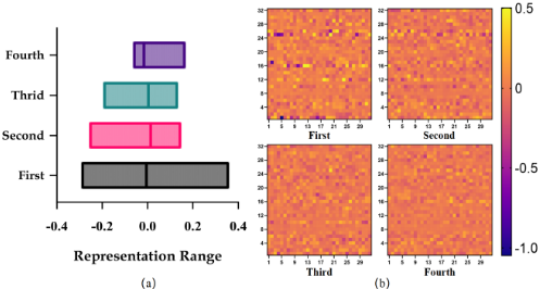
First, the number of learnable parameters increases substantially as the number of layers and channels of convolution increases in pansharpening problem. But few works in this field focus on lightweight network design, which aims to reduce the scale of parameters by a large amount compared to SOTA approaches. Furthermore, principal component analysis (PCA) demonstrates that not all parameters are fully utilized. Fig. 2 shows that the channels of the standard convolution kernel correlate with each other, resulting in redundancy, which further reduces the efficiency of the network and causes huge computational costs and memory storage.
Second, though BSConv [Haase and Amthor2020] can cut down the parameters by generating a convolution kernel via a "blueprint" and a set of weights, it only has linear representation capability, which restricts the feature extraction ability of BSConv as a general module in CNN. Fig. 3 shows that the BSConv can only span a linear subspace while both the standard convolution and LGPConv are distributed in the whole kernel space.
Third, the above two items motivate us to use the advantage of BSConv to maintain low-scale parameters while taking nonlinearity and randomness into consideration in the design of pansharpening network (see Fig. 1). Since Gaussian distribution is a commonly existing distribution of random variables, it can approximate the probability distribution of the randomness among channels. Thus, generating random perturbations by Gaussian noise is reasonable while considering the correlation among channels.
3 Method
3.1 Learnable Gaussian Perturbation Convolution
In this section, we propose a novel convolution operation named Learnable Gaussian Perturbation Convolution (LGPConv). To extract key information from feature maps, LGPConv employs the Learnable Gaussian Perturbation Kernel (LGPKernel, see Fig. 1), generated based on the premier kernel (see the following) and noise perturbations. Specifically, the premier kernel is presented as a template considering channel correlations. Furthermore, Gaussian perturbation is used to achieve channel randomization and nonlinear representation.
The preparation of linear algebra. To illustrate the given method, we need to first present some basic concepts in linear algebra, which can be found from the book in [Meyer2000]. Definition 1. If a set α = {α1, · · · , αr} where αi ∈ Rn , and the r vectors are independent, then α can span a subspace M of Rn .
Definition 2. Suppose ˜α = {˜α1, · · · , ˜αm} where ˜αi ∈ Rn , and all vectors in ˜α are independent. If m ≥ r, then ˜α can represent the subspaceM. Otherwise, ˜α can not represent the subspace M.
The premier kernel. As shown in Fig. 2, different channels in a standard kernel have a high degree of correlation, resulting in redundancy and computational inefficiency. The premier kernel, inspired by BSConv [Haase and Amthor2020], can simplify the kernel of the standard convolution. As shown in Fig. 4, the premier kernel for ith output channel mainly composes of a "blueprint" kernel Bi ∈ RK×K and a set of corresponding weights ki ∈ RCin . Thus, the convolution based on the premier kernel ˜wi can be represented as:
where yi is ith output channel, and xm,m ∈ {1, · · · ,Cin}, denotes the input tensor. The generation of the premier kernel is two operations in sequence, i.e., pointwise convolution and depthwise convolution. The premier kernel, on the other hand, just analyzes the similarity among channels, ignoring randomness and nonlinearity. In the following, we will give out the relevant mathematical explanations and introduce the solution for the premier kernel's limitations, i.e., Gaussian perturbation.
Definition 3. For easy analysis, we can reshape the wi ∈ RK×K×Cin to Cin vectors vi ∈ RK2 . The following kernel set is defined as,
where vi are distributed as points in RK2 space.
Based on Def. 1 and Def. 3, the standard kernel wi with K2 independent vectors can represent a kernel space RK2 . However, the premier kernel ˜wi is linear along the channel dimension. The premier kernel contains Cin points in RK2 space (actually located on a line, see an example in Fig. 3 (c)), and is just a subspace of RK2 , according to Def. 2.
Gaussian Perturbation. The premier kernel only considers the correlation among channels and simplifies the standard kernel by a linear transformation, limiting the kernel's representation capability. To achieve the nonlinearity among all channels, we apply random perturbation to increase randomness, thus expanding the representation range of the premier kernel. Formally, the newly designed kernel is the sum of the premier kernel and the random bias.
where ηi = [η1 i , η2 i , · · · , ηCin i ] ∈ RK×K×Cin can be viewed as Cin independent vectors with the size of K2 × 1 according to Def. 1. Based on Eq. 2 and Eq. 8, we can rewrite the formulation of convolution operation for the i-th output channel as follows,
In the following part, we will demonstrate how to generate ηi. As one type of commonly existing noise, Gaussian noise can produce multiple independent and identically distributed (i.i.d) vectors, which have a probability density function equal to that of the normal distribution. The probability density function p of a Gaussian random variable ϵ is shown as,
where µ and σ are the mean and standard deviation.
Due to the random and independent nature of Gaussian noise, we use it to generate a group of ηi, named Gaussian perturbation, see as follows,
where ϵ is a tensor of Gaussian random variables and H(·) denotes the operations of generating Gaussian perturbation. Given the variety of possible options for H(·), the simplest depthwise and pointwise convolutions in sequence are chosen for cutting down the parameters in this work. Because of the randomness of noise, H(ϵ) can be generated in RCout×K×K×Cin , which includes multiple independent vectors. Thus, Gaussian perturbation based on η can extend across the entire kernel space.
Though Gaussian perturbation has the same size as the premier kernel, it is independent and random in the kernel space, alleviating the constraints imposed by the linearity of the premier kernel. By injecting Gaussian perturbation into the premier kernel, we obtain the LGPKernel as the following,
According to Def. 1 and Def. 3, it can be deduced that LGPKernel can represent the kernel space RK2 and extract additional rich features.
Implementation of LGPConv. To sum up, as Fig. 4 shows, the input feature map is initially extracted using the premier kernel in a convolution process. Then the output is fed into the Gaussian perturbation through convolution operation. Following that, the outputs of two processes (i.e., the convolution based on premier kernel and Gaussian perturbation) are added, and the entire procedure can be summarized as follows,
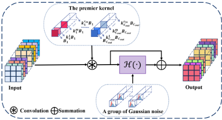
LGPConv can reduce parameters from Cout ×K×K×Cin to Cout × (2K2 + 2Cin) using Eq. 13. See the parameter comparison in Tab. 1.
| Convolution Type | Parameters |
|---|---|
| Standard Conv | Cout × K × K × Cin |
| BSConv [Haase and Amthor2020] | Cout × (K2 +Cin) |
| LGPConv | Cout × (2K2 + 2Cin) |
3.2 Architecture of LGPConv-based Pansharpening Network (LGPConv-Net)
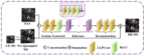
We propose the network for pansharpening, i.e., LGPConvNet, where all convolutions are realized by LGPConv. In Fig. 5, the proposed network has three simple components, i.e., an initial feature extractor, a deep inference block, and a fusion reconstruction. More details please see supplementary.
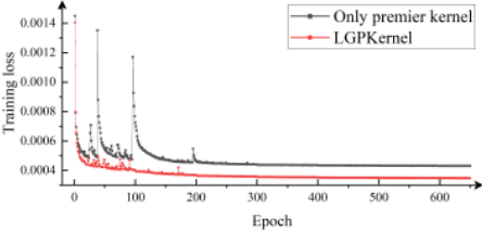
Figure 6: Convergence comparison when using only premier kernel and LGPKernel.
Training process uses a simple ℓ1 loss to minimize the difference between the predicted image ˜Mi and the ground truth Mgt,i ,
where N is the sample number, and ∥ · ∥1 is the ℓ1 norm.
3.3 Mathematical Explanations: Convergence Analysis with Lipschitz Condition
Recent research has demonstrated that the Lipschitz constant can be utilized to demonstrate the robustness of DL-based networks [Liu et al.2018,Hein and Andriushchenko2017,Weng et al.2018]. In this paper, we use it to explain that the training of LGPConv-Net is equivalent to Lipschitz regularization, which further explains the convergence of the proposed network. The Lipschitz constant of LGPConv-Net is given as the following definition.
Definition 4. For the network with specific perturbation, we define the loss function as ℓϵ that has a Lipschitz constant Lℓϵ . Also we have the following inequality,
Although LGPConv contains Gaussian perturbation, a theoretical convergence analysis shows it is still robust. Then, we demonstrate that our network can regulate the Lipschitz constant by expanding the expectation function,
In Eq. 16, we employ Taylor expansion at ϵ = 0 and retain only the second-order term because the variance of Gaussian random variables is relatively small in default. By noticing the Gaussian vector ϵ is i.i.d with mean µ and the quadratic term is directly dependent on variance of noise and the trace of Hessian, Eq. 16 can be formulated as,
| Method | SAM(±std)↓ | ERGAS(±std)↓ | SCC(±std)↑ | Q8(±std)↑ | Params | GFLOPS | A.T. |
|---|---|---|---|---|---|---|---|
| BDSD [Garzelli et al.2007] | 6.9997±2.8530 | 5.1670±2.2475 | 0.8712±0.0798 | 0.8126±0.1234 | - | - | 0.0151 |
| MTF_GLP_CBD [Aiazzi et al.2006] | 5.2861±1.9582 | 4.1627±1.7748 | 0.8904±0.0698 | 0.8540±0.1144 | - | - | 0.0161 |
| CVPR19 [Fu et al.2019] | 5.2058±1.8688 | 5.1411±2.1191 | 0.8667±0.0604 | 0.7927±0.1228 | - | - | 1.5844 |
| PanNet [Yang et al.2017] | 4.0921±1.2733 | 2.9524±0.9778 | 0.9495±0.0461 | 0.8942±0.1170 | 83K | 0.340 | 0.0025 |
| PNN [Masi et al.2016b] | 4.0015±1.3292 | 2.7283±1.0042 | 0.9515±0.0465 | 0.9083±0.1122 | 104K | 0.299 | 0.0011 |
| DiCNN [He et al.2019] | 3.9805±1.3292 | 2.7367±1.0156 | 0.9517±0.0472 | 0.9097±0.1170 | 47K | 0.192 | 0.0005 |
| DMDNet [Fu et al.2020] | 3.9714±1.2482 | 2.8572±0.9663 | 0.9527±0.0447 | 0.9000±0.1142 | 100K | 0.359 | 0.0043 |
| FusionNet [Deng et al.2021] | 3.7435±1.2259 | 2.5679±0.9442 | 0.9580±0.0450 | 0.9135±0.1122 | 79k | 0.323 | 0.0022 |
| LPPN [Jin et al.2022a] | 3.9021±1.2901 | 2.6404±0.9600 | 0.9552±0.0450 | 0.9130±0.1110 | 51k | 1.285 | 0.0051 |
| LGPConv-Net | 3.5940±1.2141 | 2.4560±0.9295 | 0.9596±0.0446 | 0.9161±0.1107 | 27K | 0.112 | 0.0034 |
As a convex relaxation, if we assume ℓ0(θ) is convex, then Eq. 17 can be formulated as follows according to Def. 4.,
which indicates that the training of LGPConv-Net is equivalent to training the network without perturbation and an extra regularization of the Lipschitz constant. By controlling both mean and variance of Gaussian noise, we can balance the convergence of LGPConv-Net. The training loss curves for only using the premier kernel and LGPConv are shown in Fig. 6. It can be observed that huge fluctuations exist when having no Gaussian perturbation (i.e., only premier kernel), while LGPConv holds a steady loss convergence.
4 Experiments
Due to the page limitation, dataset, metrics, compared methods, and training platform are mentioned in supplementary.
4.1 Assessment on 8-band and 4-band Dataset
In Tab. 2, we show the average quantitative results of different methods on the 1258 samples from WV-3 dataset with eight bands. The proposed LGPConv-Net clearly has the best performance and the fewest computational costs (parameters and GFLOPS) compared to all other methods simultaneously. Furthermore, we exhibit the average inference time for each fusion method, denoted as A.T. in seconds. We also assess the proposed method on 4-band datasets, i.e., GF-2 and QB data. The quantitative results in terms of all compared methods are shown in Tab. 3. As can be seen, LGPConv-Net outperforms other competing methods with lower SAM and ERGAS and higher Q4 and SCC, which proves that the proposed LGPConvNet can tackle with 4-band dataset efficiently while maintaining the smallest parameter scale. For visual comparisons, please refer to supplementary material.
4.2 Discussion
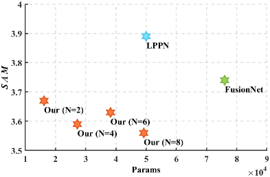
The number of Resnet-like blocks in LGPConv-Net. Since we have set the number of Resnet-like blocks (N) to 4 in default, the influence of Resnet-like blocks will be demonstrated by justifying its number. We have tested the performance of LGPConv-Net with the different number of Resnet-like blocks in the deep inference block, where N = 2, 4, 6, 8. The experiments are only conducted on WV-3 dataset in the discussion. As Fig. 7 shows, all the LGPConv-Net with varying N have good performance and all outperform LPPN [Jin et al.2022a] and FusionNet [Deng et al.2021] with less parameters. Though there are fluctuations with N increasing, N = 4 is an economical choice.
Gaussian perturbation and Gaussian noise. In this section, we assess the effectiveness of Gaussian perturbation and the corresponding Gaussian noise in LGPConv. In order to illustrate this, we design the following three cases to compare and the results are shown in Tab. 4 (the standard error is omitted for page limiting). LGPKernel outperforms the other two by replacing all LGPKernel with the premier kernel and LGPKernel without (w/o) the Gaussian noise. Thus, both Gaussian perturbation and Gaussian noise are indispensable for LGPKernel. Different convolution types. Three different convolutional operations, i.e., standard convolution, BSConv [Haase and Amthor2020], and LGPConv, are embedded into the proposed network (Fig. 5). Since the parameters of BSConv are less than LGPConv, the number of Resnet-like blocks (N) is added to 10 for a fair comparison. As shown in Tab. 5, though standard convolution and BSConv-based network consume more parameters than LGPConv, the proposed LGPConv still obtains the best performance among all. Therefore, LGPConv has addressed the existing problems for standard convolution and BSConv, i.e., reducing the scale of parameter and enlarging the representation range simultaneously.
| (a) 81 samples from GF-2 dataset | (b) 48 samples from QB dataset | ||||||||
|---|---|---|---|---|---|---|---|---|---|
| Method | SAM(±std)↓ | ERGAS(±std)↓ | SCC(±std)↑ | Q4(±std)↑ | SAM(±std)↓ | ERGAS(±std)↓ | SCC(±std)↑ | Q4(±std)↑ | Params |
| BDSD [Garzelli et al.2007] | 2.29±0.66 | 2.07±0.61 | 0.87±0.05 | 0.87±0.04 | 7.75±1.93 | 7.46±0.99 | 0.85±0.06 | 0.70±0.12 | - |
| MTF_GLP_CBD [Aiazzi et al.2006] | 2.26±0.72 | 2.02±0.60 | 0.87±0.05 | 0.87±0.04 | 7.67±1.88 | 7.42±0.97 | 0.85±0.06 | 0.65±0.14 | - |
| CVPR19 [Fu et al.2019] | 2.15±0.50 | 2.24±0.64 | 0.87±0.04 | 0.86±0.02 | 7.69±1.84 | 9.15±1.52 | 0.82±0.04 | 0.55±0.19 | - |
| PanNet [Yang et al.2017] | 1.39±0.32 | 1.22±0.28 | 0.95±0.01 | 0.94±0.02 | 5.31±0.99 | 5.23±0.54 | 0.93±0.06 | 0.82±0.08 | 78K |
| PNN [Masi et al.2016b] | 1.45±0.36 | 1.27±0.32 | 0.94±0.02 | 0.94±0.02 | 5.20±0.95 | 4.87±0.46 | 0.93±0.05 | 0.83±0.07 | 80K |
| DiCNN [He et al.2019] | 1.49±0.38 | 1.32±0.35 | 0.94±0.02 | 0.94±0.02 | 5.30±0.99 | 5.23±0.54 | 0.92±0.05 | 0.81±0.08 | 43K |
| DMDNet [Fu et al.2020] | 1.29±0.31 | 1.12±0.26 | 0.96±0.01 | 0.95±0.02 | 5.11±0.94 | 4.74±0.65 | 0.94±0.06 | 0.83±0.07 | 98K |
| FusionNet [Deng et al.2021] | 1.18±0.27 | 1.00±0.22 | 0.97±0.01 | 0.96±0.01 | 5.31±1.02 | 5.16±0.68 | 0.93±0.05 | 0.82±0.08 | 76k |
| LPPN [Jin et al.2022a] | 1.34±0.25 | 1.05±0.22 | 0.96±0.01 | 0.96±0.02 | 4.84±0.83 | 4.61±0.88 | 0.95±0.05 | 0.84±0.07 | 160K |
| LGPConv-Net | 1.17±0.28 | 0.98±0.24 | 0.97±0.01 | 0.97±0.02 | 4.42±0.74 | 3.70±0.27 | 0.96±0.05 | 0.86±0.06 | 27K |
| Kernel Type | SAM↓ | ERGAS↓ | SCC↑ | Q8↑ |
|---|---|---|---|---|
| Only premier kernel | 4.064 | 2.796 | 0.950 | 0.905 |
| LGPKernel w/o Gaussian noise | 3.823 | 2.607 | 0.956 | 0.913 |
| LGPKernel | 3.594 | 2.456 | 0.961 | 0.918 |
| Convolution Type | SAM↓ | ERGAS↓ | SCC↑ | Q8↑ | N | Params |
|---|---|---|---|---|---|---|
| Standard Conv | 3.803 | 2.593 | 0.956 | 0.914 | 4 | 87K |
| BSConv [Haase and Amthor2020] | 3.845 | 2.857 | 0.952 | 0.910 | 10 | 29K |
| LGPConv | 3.594 | 2.456 | 0.961 | 0.918 | 4 | 27K |
| σ1 | σ2 | SAM↓ | ERGAS↓ | SCC↑ | Q8↑ |
|---|---|---|---|---|---|
| 0.003 | 0.005 | 3.695 | 2.513 | 0.959 | 0.915 |
| 0.001 | 0.005 | 3.665 | 2.515 | 0.959 | 0.915 |
| 0.005 | 0.003 | 3.615 | 2.485 | 0.960 | 0.918 |
| 0.005 | 0.001 | 3.650 | 2.505 | 0.960 | 0.917 |
| 0.005 | 0.005 | 3.594 | 2.456 | 0.961 | 0.918 |
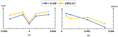
The initial distribution of Gaussian noise. As mentioned in the accomplishment of LGPConv, Gaussian noise is the key input for generating Gaussian perturbation, and depthwise and pointwise convolutions are used in sequence for parameter reduction. Thus, there are two sets of Gaussian noise for both depthwise and pointwise convolutions. Next, we will examine how the initial distributions, i.e., µ and σ, affect the performance of LGPConv-Net. First, considering the Gaussian noise for depthwise and pointwise convolutions follows different initial distributions, i.e., N(µ1, σ2 1 ) and N(µ2, σ2 2 ), respectively. For easier analysis, we set the µ1 = µ2 = 0 as the default. Tab. 6 demonstrates that optimal performance is achieved when the initial distributions are identical. Then, the impact of µ and σ will be tested with two sets of Gaussian noise, whose initial distributions are identical. Fig. 8 (a) shows that µ = 0 has the best outcomes. From Fig. 8 (b), the results have improved with σ increasing, which indicates that the initial distribution of Gaussian noise is valid and our LGPConv-Net is robust to the perturbation.
5 Conclusion
Standard convolution is highly redundant due to the unawareness of channel-across correlations. We propose a novel convolution, i.e., LGPConv, which consists of he premier kernel and Gaussian perturbation. The premier kernel effectively reduces the parameters by considering the similarity among channels, while Gaussian perturbation promises the randomness and nonlinearity of the LGPKernel. Based on the LGPConv, a simple end-to-end network, i.e., LGPConv-Net, is designed for pansharpening task. Extensive experiments show the prominent performance of LGPConv-Net in terms of quantitative and visual results, while only requiring a very minor scale of parameters to the best of our knowledge. Also, our method has relatively limited generalization, this may be due to Gaussian random perturbation, and it is more sensitive to the distribution changes of datasets acquired by different sensors.
@inproceedings{ijcai2023p517,
  title     = {LGPConv: Learnable Gaussian Perturbation Convolution for Lightweight Pansharpening},
  author    = {Zhao, Chen-Yu and Zhang, Tian-Jing and Ran, Ran and Chen, Zhi-Xuan and Deng, Liang-Jian},
  booktitle = {Proceedings of the Thirty-Second International Joint Conference on
               Artificial Intelligence, {IJCAI-23}},
  publisher = {International Joint Conferences on Artificial Intelligence Organization},
  editor    = {Edith Elkind},
  pages     = {4647--4655},
  year      = {2023},
  month     = {8},
  note      = {Main Track},
  doi       = {10.24963/ijcai.2023/517},
  url       = {https://doi.org/10.24963/ijcai.2023/517},
}
TY - CPAPER TI - LGPConv: Learnable Gaussian Perturbation Convolution for Lightweight Pansharpening AU - Zhao, Chen-Yu AU - Zhang, Tian-Jing AU - Ran, Ran AU - Chen, Zhi-Xuan AU - Deng, Liang-Jian T2 - Proceedings of the Thirty-Second International Joint Conference on Artificial Intelligence, IJCAI-23 PB - International Joint Conferences on Artificial Intelligence Organization PY - 2023 SP - 4647 EP - 4655 DO - 10.24963/ijcai.2023/517 UR - https://doi.org/10.24963/ijcai.2023/517 ER -Copied
Machine-readable versions of this paper, for tools and AI agents:





