
K∗ Search over Orbit Space for Top-k Planning
Proceedings of the Thirty-Second International Joint Conference on Artificial Intelligence. Main Track. Pages 5368-5376.
https://doi.org/10.24963/ijcai.2023/596
Keywords
- Planning and Scheduling: PS: Search in planning and scheduling
- Planning and Scheduling: PS: Planning algorithms
- Planning and Scheduling: PS: Theoretical foundations of planning
Abstract
Top-k planning, the task of finding k top-cost plans, is a key formalism for many planning applications and K* search is a well-established approach to top-k planning. The algorithm iteratively runs A* search and Eppstein’s algorithm until a sufficient number of plans is found. The performance of K* algorithm is therefore inherently limited by the performance of A*, and in order to improve K* performance, that of A* must be improved. In cost-optimal planning, orbit space search improves A* performance by exploiting symmetry pruning, essentially performing A* in the orbit space instead of state space. In this work, we take a similar approach to top-k planning. We show theoretical equivalence between the goal paths in the state space and in the orbit space, allowing to perform K* search in the orbit space instead, reconstructing plans from the found paths in the orbit space. We prove that our algorithm is sound and complete for top-k planning and empirically show it to achieve state-of-the-art performance, overtaking all existing to date top-k planners. The code is available at https://github.com/IBM/kstar.
- [Aljazzar and Leue, 2011] Husain Aljazzar and Stefan Leue. K*: A heuristic search algorithm for finding the k shortest paths. Artificial Intelligence, 175(18):2129-2154, 2011.
- [Alkhazraji et al., 2014] Yusra Alkhazraji, Michael Katz, Robert Mattmüller, Florian Pommerening, Alexander Sh- leyfman, and Martin Wehrle. Metis: Arming Fast Down- ward with pruning and incremental computation. In Eighth International Planning Competition (IPC-8): Planner Ab- stracts, pages 88-92, 2014.
- [Bäckström and Nebel, 1995] Christer Bäckström and Bern- hard Nebel. Complexity results for SAS + planning. Com- putational Intelligence, 11(4):625-655, 1995.
- [Boddy et al., 2005] Mark Boddy, Johnathan Gohde, Tom Haigh, and Steven Harp. Course of action generation for cyber security using classical planning. In Susanne Bi- undo, Karen Myers, and Kanna Rajan, editors, Proceed- ings of the Fifteenth International Conference on Auto- mated Planning and Scheduling (ICAPS 2005), pages 12- 21. AAAI Press, 2005.
- [Domshlak et al., 2012a] Carmel Domshlak, Michael Katz, and Sagi Lefler. Landmark-enhanced abstraction heuris- tics. Artificial Intelligence, 189:48-68, 2012.
- [Domshlak et al., 2012b] Carmel Domshlak, Michael Katz, and Alexander Shleyfman. Enhanced symmetry breaking in cost-optimal planning as forward search. In Lee Mc- Cluskey, Brian Williams, José Reinaldo Silva, and Blai Bonet, editors, Proceedings of the Twenty-Second Interna- tional Conference on Automated Planning and Scheduling (ICAPS 2012), pages 343-347. AAAI Press, 2012.
- [Domshlak et al., 2015] Carmel Domshlak, Michael Katz, and Alexander Shleyfman. Symmetry breaking in deter- ministic planning as forward search: Orbit space search algorithm. Technical Report IS/IE-2015-03, Technion, 2015.
- [Emerson and Sistla, 1996] E. Allen Emerson and A. Prasad Sistla. Symmetry and model checking. Formal Methods in System Design, 9(1-2):105-131, 1996.
- [Eppstein, 1998] David Eppstein. Finding the k shortest paths. SIAM Journal on Computing, 28(2):652-673, 1998.
- [Haslum et al., 2007] Patrik Haslum, Adi Botea, Malte Helmert, Blai Bonet, and Sven Koenig. Domain- independent construction of pattern database heuristics for cost-optimal planning. In Proceedings of the Twenty- Second AAAI Conference on Artificial Intelligence (AAAI 2007), pages 1007-1012. AAAI Press, 2007.
- [Helmert and Domshlak, 2009] Malte Helmert and Carmel Domshlak. Landmarks, critical paths and abstractions: What's the difference anyway? In Alfonso Gerevini, Adele Howe, Amedeo Cesta, and Ioannis Refanidis, ed- itors, Proceedings of the Nineteenth International Con- ference on Automated Planning and Scheduling (ICAPS 2009), pages 162-169. AAAI Press, 2009. Helmert et al., 2007] Malte Helmert, Patrik Haslum, and Jörg Hoffmann. Flexible abstraction heuristics for op- timal sequential planning. In Mark Boddy, Maria Fox, and Sylvie Thiébaux, editors, Proceedings of the Seven- teenth International Conference on Automated Planning and Scheduling (ICAPS 2007), pages 176-183. AAAI Press, 2007.
- [Helmert, 2006] Malte Helmert. The Fast Downward plan- ning system. Journal of Artificial Intelligence Research, 26:191-246, 2006.
- [Junttila and Kaski, 2007] Tommi Junttila and Petteri Kaski. Engineering an efficient canonical labeling tool for large and sparse graphs. In Proceedings of the Ninth Workshop on Algorithm Engineering and Experiments (ALENEX 2007), pages 135-149. SIAM, 2007.
- [Katz and Lee, 2023] Michael Katz and Junkyu Lee. K * and partial order reduction for top-quality planning. In Pro- ceedings of the 16th Annual Symposium on Combinatorial Search (SoCS 2023). AAAI Press, 2023.
- [Katz et al., 2018a] Michael Katz, Shirin Sohrabi, Horst Samulowitz, and Silvan Sievers. Delfi: Online planner se- lection for cost-optimal planning. In Ninth International Planning Competition (IPC-9): Planner Abstracts, pages 57-64, 2018.
- [Katz et al., 2018b] Michael Katz, Shirin Sohrabi, Octavian Udrea, and Dominik Winterer. A novel iterative approach to top-k planning. In Mathijs de Weerdt, Sven Koenig, Gabriele Röger, and Matthijs Spaan, editors, Proceed- ings of the Twenty-Eighth International Conference on Au- tomated Planning and Scheduling (ICAPS 2018), pages 132-140. AAAI Press, 2018.
- [Katz et al., 2020] Michael Katz, Parikshit Ram, Shirin Sohrabi, and Octavian Udrea. Exploring context-free lan- guages via planning: The case for automating machine learning. In J. Christopher Beck, Erez Karpas, and Shirin Sohrabi, editors, Proceedings of the Thirtieth Interna- tional Conference on Automated Planning and Scheduling (ICAPS 2020), pages 403-411. AAAI Press, 2020.
- [Lee et al., 2023] Junkyu Lee, Michael Katz, and Shirin Sohrabi. On K * search for top-k planning. In Proceedings of the 16th Annual Symposium on Combinatorial Search (SoCS 2023). AAAI Press, 2023.
- [Luks, 1993] Eugene M. Luks. Permutation groups and polynomial-time computation. In Groups and Computa- tion, volume 11 of DIMACS Series in Discrete Mathe- matics and Theoretical Computer Science, pages 139-175. 1993.
- [Pochter et al., 2011] Nir Pochter, Aviv Zohar, and Jeffrey S. Rosenschein. Exploiting problem symmetries in state- based planners. In Wolfram Burgard and Dan Roth, ed- itors, Proceedings of the Twenty-Fifth AAAI Conference on Artificial Intelligence (AAAI 2011), pages 1004-1009. AAAI Press, 2011.
- [Riabov and Liu, 2006] Anton V. Riabov and Zhen Liu. Scalable planning for distributed stream processing sys- tems. In Derek Long, Stephen F. Smith, Daniel Bor- rajo, and Lee McCluskey, editors, Proceedings of the Six- teenth International Conference on Automated Planning and Scheduling (ICAPS 2006), pages 31-40. AAAI Press, 2006.
- [Riabov et al., 2014] Anton V. Riabov, Shirin Sohrabi, and Octavian Udrea. New algorithms for the top-k planning problem. In ICAPS 2014 Scheduling and Planning Appli- cations woRKshop, pages 10-16, 2014.
- [Seipp and Helmert, 2018] Jendrik Seipp and Malte Helmert. Counterexample-guided Cartesian abstrac- tion refinement for classical planning. Journal of Artificial Intelligence Research, 62:535-577, 2018.
- [Shleyfman and Jonsson, 2021] Alexander Shleyfman and Peter Jonsson. Computational complexity of computing symmetries in finite-domain planning. Journal of Artifi- cial Intelligence Research, 70:183-1221, 2021.
- [Shleyfman et al., 2015] Alexander Shleyfman, Michael Katz, Malte Helmert, Silvan Sievers, and Martin Wehrle. Heuristics and symmetries in classical planning. In Blai Bonet and Sven Koenig, editors, Proceedings of the Twenty-Ninth AAAI Conference on Artificial Intelligence (AAAI 2015), pages 3371-3377. AAAI Press, 2015.
- [Sievers and Katz, 2018] Silvan Sievers and Michael Katz. Metis 2018. In Ninth International Planning Competition (IPC-9): Planner Abstracts, pages 83-84, 2018.
- [Sievers et al., 2017] Silvan Sievers, Martin Wehrle, Malte Helmert, and Michael Katz. Strengthening canonical pat- tern databases with structural symmetries. In Alex Fuku- naga and Akihiro Kishimoto, editors, Proceedings of the 10th Annual Symposium on Combinatorial Search (SoCS 2017), pages 91-99. AAAI Press, 2017.
- [Sohrabi et al., 2016] Shirin Sohrabi, Anton V. Riabov, Oc- tavian Udrea, and Oktie Hassanzadeh. Finding diverse high-quality plans for hypothesis generation. In Gal A. Kaminka, Maria Fox, Paolo Bouquet, Eyke Hüllermeier, Virginia Dignum, Frank Dignum, and Frank van Harme- len, editors, Proceedings of the 22nd European Conference on Artificial Intelligence (ECAI 2016), pages 1581-1582. IOS Press, 2016.
- [Sohrabi et al., 2018] Shirin Sohrabi, Anton V. Riabov, Michael Katz, and Octavian Udrea. An AI planning solu- tion to scenario generation for enterprise risk management. In Proceedings of the Thirty-Second AAAI Conference on Artificial Intelligence (AAAI 2018), pages 160-167. AAAI Press, 2018.
- [Speck et al., 2020] David Speck, Robert Mattmüller, and Bernhard Nebel. Symbolic top-k planning. In Vincent Conitzer and Fei Sha, editors, Proceedings of the Thirty- Fourth AAAI Conference on Artificial Intelligence (AAAI 2020), pages 9967-9974. AAAI Press, 2020.
- [Wehrle and Helmert, 2012] Martin Wehrle and Malte Helmert. About partial order reduction in planning and computer aided verification. In Lee McCluskey, Brian Williams, José Reinaldo Silva, and Blai Bonet, editors, Proceedings of the Twenty-Second International Con- ference on Automated Planning and Scheduling (ICAPS 2012), pages 297-305. AAAI Press, 2012.
References were extracted automatically from the PDF and may contain errors.
Full text extracted automatically from the PDF; figures, tables and equations may differ. The PDF is the version of record.
1 Introduction
Top-k planning is essential to many planning applications, including malware detection [Boddy et al., 2005], hypothesis generation [Sohrabi et al., 2016], scenario planning [Sohrabi et al., 2018], and machine learning pipeline generation [Katz et al., 2020]. There are currently three main approaches to top-k planning. The last one chronologically is based on a so-called symbolic search [Speck et al., 2020]. Another approach to top-k planning is called Forbid Iterative (FI). It is based on iteratively reformulating the input task, excluding the previously found plans from the task plans space [Katz et al., 2018b]. The third approach is based on a K∗ search [Aljazzar and Leue, 2011]. In planning, it was first implemented within a planner for an SPPL language [Riabov and Liu, 2006], with some simplifications [Riabov et al., 2014]. Later, a similar variant was implemented within a PDDL planner [Katz et al., 2018b], and most recently the original variant of Aljazzar and Leue [2011] was implemented on top of a PDDL planner [Lee et al., 2023]. That last variant significantly improves the performance of K∗ search, compared to the previous one and for the first time allows for using inconsistent heuristics. It works in two interchanging phases, A∗ search and Eppstein's k shortest paths algorithm [Eppstein, 1998] on the developed search space. Thus, the performance of K∗ algorithm is inherently limited by that of A∗ and in order to improve K∗ performance, one must improve A∗ .
In cost-optimal planning, the issue of A∗ performance was tackled, among other, by using search space pruning techniques. Two main such techniques are partial order reduction [Wehrle and Helmert, 2012] and symmetry based search pruning [Pochter et al., 2011; Domshlak et al., 2012b]. For the latter, two search algorithms were suggested, DKS [Domshlak et al., 2012b] and orbit space search (OSS) [Domshlak et al., 2015]. While DKS performs the search in problem state space, pruning states that deem symmetric to the previously encountered ones, OSS is essentially performing A∗ search in a so-called orbit space instead of the state space. In the orbit space, nodes correspond to equivalence classes of states, with the equivalence relation based on detecting states as symmetric. In both algorithms, the symmetry detection is done via so-called canonical states. While there is no clear dominance of one of the methods over the other, DKS requires storing two states per search node, the actual state and the canonical one. OSS, on the other hand, requires only storing the canonical state. Thus, in principle, it should have a smaller memory consumption.
In this work, we take a similar approach to top-k planning. First, as K∗ requires transforming the input planning task into a task with a single goal state, we propose a transformation into a planning task with a single goal state that preserve the symmetries of the input task. Next, focusing on the orbit space search, we establish the theoretical grounds for performing K∗ search in the orbit space. We do that by showing the equivalence between the goal paths in the state space and the orbit space. These goal paths in the orbit space can then be cast into actual plans. We then prove that our suggested algorithm is sound and complete for top-k planning. Last, we perform an extensive empirical evaluation of the proposed algorithm with a variety of admissible heuristics, both consistent and inconsistent, and comparing to all existing top-k planners. Our evaluation shows the new approach to be competitive with the current state-of-the-art.
2 Background
This section introduces necessary concepts in top-k planning, K∗ search algorithm for top-k planning, and OSS for cost optimal planning.
2.1 Top-k Classical Planning
A planning task Π = 〈V,O, s0 , s⋆ 〉 in SAS+ formalism [B¨ackstr¨om and Nebel, 1995] consists of a finite set of finitedomain state variables V, a finite set of actions O, an initial state s0, and the goal s⋆. Each variable v ∈ V is associated with a finite domain dom(v) of values. An assignment of a value d ∈ dom(v) to a variable v ∈ V denoted by a pair 〈v, d〉 is called fact, and the set of all facts is denoted by F . A partial assignment p maps a subset of variables vars(p) ⊆ V to values in their domains. For a variable v ∈ V and partial assignment p, the value of v in p is denoted by p[v] if v ∈ vars(p) and we say p[v] is undefined otherwise. A full assignment s is called a state, and the set of all states is denoted by S. State s is consistent with a partial assignment p if they agree on all variables in vars(p), denoted by p ⊆ s. Each action o in O is a pair 〈pre(o), eff (o)〉, where pre(o) and eff (o) are partial assignments called precondition and effect. Further, o has an associated non-negative cost denoted by cost(o) ∈ R0+. An action o is applicable in state s if pre(o) ⊆ s. Applying o in s results in a state denoted by sJoK, where sJoK[v] = eff (o)[v] for all v ∈ vars(eff ) and sJoK[v] = s[v] for all other variables. An action sequence π = 〈o1, . . . , on〉 is applicable in state s if there are states 〈s0, . . . , sn〉 such that oi is applicable in si-1 and si-1JoiK = si for 0 ≤ i ≤ n. We denote sn by sJπK. An action sequence with s⋆ ⊆ s0JπK is called a plan. The cost of a plan π, denoted by cost(π) is the summed cost of the actions in the plan. The set of all plans is denoted by PΠ, and an optimal plan is a plan in PΠ with the lowest cost.
Example 1 (Gripper Task). We will use a famous gripper task introduced by Jana Koehler as a running example throughout the paper. There is a robot R with two grippers l and r, and each can carry a ball. The goal is to move four balls, b1, b2, b3, b4, from room A to room B.
- A state can be represented by seven SAS+variables: one variable R with dom(R) = {A, B} for encoding the location of the robot, four variables, {bi|i ∈ [1..4]} with dom(bi) = {A, B, R} for encoding the location of the four balls, and two variables, l and r for grippers with domain {E, b1, b2, b3, b4} for encoding the object a gripper holds, where E represents holding nothing.
- For brevity, we denote a state with five letters, comprising the location of the robot and four balls. Namely, ARLBB stands for a state with facts: 〈R, A〉, 〈b1, r〉, 〈b2, l〉, 〈b3, B〉, 〈b4, B〉, 〈l, b2〉, and 〈r, b1〉.
- Actions are pick, drop, and move for manipulating the balls and moving between rooms, abbreviated as follows. P1LA denotes a pick action taking b1 with the left gripper in room A, D2RB denotes a drop action dropping b2 from the right gripper in room B, MAB denotes a move action moving from room A to B, etc.
Next, we present the top-k planning problem, as defined by Sohrabi et al.; Katz et al. [2016; 2018b].
Definition 1 (top-k planning problem). Given a classical planning task Π and a natural number k, top-k planning problem is finding a set of plans P ⊆ PΠ satisfying the following properties.
- For all plans π ∈ P, if there exists a plan π′ ∈ PΠ such that C(π′ ) < C(π), then π′ ∈ P,
We say a top-k planning problem 〈Π, k〉 is solvable if |P| = k and unsolvable if |P| < k. Note that cost-optimal planning is a special case of top-k planning for k = 1.
2.2 K∗ Search for Top-k Planning
Given a top-k planning problem 〈Π, k〉, K∗ applies Eppstein's algorithm (EA) to the search graph revealed by A∗ until the task is solved or proven to be unsolvable. In this section, we only review necessary concepts and refer to Aljazzar and Leue [2011] and Eppstein [1998] for details.
Single Goal State Reformulation of Planning Tasks
The fact that any state consistent to s⋆ is a goal state in a planning task Π = 〈V , O, s0 , s⋆ 〉 calls for a single goal state reformulation since K∗ assumes a single terminal node in the search graph. Katz et al. [2018b] showed such a reformulated task Πg = 〈V g ,Og , sg0 , sg⋆〉, where V g = V ∪ {vg} with a binary indicator variable vg for reaching a goal state, Og = {〈pre(o) ∪ 〈vg, 0〉, eff (o)〉|o ∈ O} ∪ {og} with a zero cost goal-achieving action og such that pre(og) = s⋆ ∪ {〈vg, 0〉} and eff (og) = {〈vi, t[vi]〉|vi ∈ vars(t)} ∪ {〈vg, 1〉} for an arbitrary full state t, sg0 = s0 ∪ {〈vg, 0〉}, and sg⋆ = eff (og).
Implicit Path Representation of Eppstein's Algorithm
A∗ explores a state transition graph TΠ=〈S, E〉 comprised of nodes associated with states S and edges E, induced by operators O, namely, {〈s, sJoK; o〉|pre(o) ∈ s ∀s ∈ S, ∀o ∈ O}. Denoting by GA∗ an explicit search graph revealed by A∗ , EA uses an implicit path representation relative to the shortest path tree TA∗ using a sequence of "side-tracked" edges (STE), the edges of GA∗ that are not in TA∗. For each STE (u, v), we can compute the deviation cost δ(u, v) against the cost of the incoming edge toward v in TA∗ by δ(u, v) = g(u)+cost(o)-g(v) iff v =uJoK. We denote an arbitrary goal reaching path from sg0 in GA∗ by ρA∗(sg0 , sg⋆), and the unique path from u to v in TA∗ by ρ∗A∗(u, v) if it exists. Then, any ρA∗(sg0 , sg⋆) can be uniquely represented by an ordered sequence of STEs, denoted by SIDETRACKS(ρA∗(sg0 , sg⋆)) = 〈(u1, v1), . . . , (uq, vq)〉, where an STE closer to sg⋆ appears earlier in the sequence. Namely, ρA∗(sg0 , sg⋆) can be reconstructed from SIDETRACKS(ρA∗(sg0 , sg⋆)) by
where ◦ concatenates edges and paths from left to right.
EA performs Dijkstra's algorithm over its own search graph, called path graph P(GA∗) in which each node represents SIDETRACKS(ρA∗(sg0 , sg⋆)) with the total deviation cost ∑qi=1 δ(ui, vi). Therefore, k-shortest paths are found in the order of their costs.
2.3 Orbit Space Search for Cost Optimal Planning
Symmetry breaking techniques [Pochter et al., 2011; Domshlak et al., 2012b; Shleyfman et al., 2015] significantly improved heuristic forward state space search for cost optimal classical planning. Given a planning task Π, and its state transition graph TΠ, a graph automorphism in the automorphism group of TΠ, denoted by Aut(TΠ), permutes states while preserving the adjacency between states. Any subgroup of Aut(TΠ) partitions the state space by orbits, which offers opportunity for pruning the search space. In this section, we introduce necessary concepts in OSS.
2.4 Structural Symmetries and Canonical States
Since state transition graphs are implicit, we find graph automorphisms from the syntactic structure of planning tasks, called structural symmetries [Shleyfman et al., 2015], and follow the definition shown in Sievers et al. [2017].
Definition 2 (Structural Symmetry). Given a planning task Π = 〈V,O, s0 , s⋆ 〉, a structural symmetry is a permutation σ : V ∪ F ∪ O → V ∪ F ∪ O with the following properties.
- σ(V)=V and σ(F)=F such that σ(〈v, d〉) = 〈v′ , d′ 〉 implies v′ =σ(v),
- σ(O)=O such that for o∈O, σ(pre(o))=pre(σ(o)), σ(eff (o))=eff (σ(o)), and cost(σ(o))=cost(o),
- σ(s⋆)=s⋆,
Note that the third property ensures that a structural symmetry σ stabilizes the goal. In practice, a set of structural symmetries can be detected by using tools for finding automorphisms of colored digraphs, such as Bliss [Junttila and Kaski, 2007]. These structural symmetries are the generators of the symmetry group Γ, a subgoup of Aut(TΠ).
Given two states s and t, it is crucial to quickly check whether s and t are symmetric or not for speeding up search. Unfortunately, finding σ ∈ Γ for s = σ(t) is PSPACE-hard [Shleyfman and Jonsson, 2021]. Instead of finding such σ, Pochter et al. [2011] proposed to use canonical form [Emerson and Sistla, 1996], which we call canonical states.
Definition 3 (Canonical States). Given a planning task Π = 〈V,O, s0 , s⋆ 〉 over the states S, and a group Γ of structural symmetries for Π, canonical state CΓ(s) of s ∈ S is a state generated by a mapping CΓ : S → S such that for all s, t ∈ S, CΓ(s) = CΓ(t) iff there exists σ ∈ Γ such that s = σ(t).
The common choice of CΓ implements a greedy search that outputs local lexicographically minimum states since finding the global minimum is NP-hard [Luks, 1993]. Nevertheless, missing to match structurally symmetric states only skips pruning symmetric states and it doesn't forfeit the soundness and completeness of search [Domshlak et al., 2012a].
Example 2 (Sturctural Symmetries in Gripper Task). Using the tools mentioned above, we can find a structural symmetries group with four generators as follows. Each of these structural symmetries is of order 2, meaning if σ(x) = y then also σ(y) = x must hold, so for brevity we describe only one of these. For unmentioned elements x, we have σ(x) = x.
- Permuting the left gripper l and the right gripper r: σlr(l) = r, ∀d ∈ dom(l), σlr(〈l, d〉) = 〈r, d〉, ∀X∈{1..4}, ∀Y∈{A, B}, σlr(PXYL) = PXYR, ∀X∈{1..4}, ∀Y∈{A, B}, σlr(DXYL) = DXYR,
- permuting balls b1 and b2: σ12(b1)=b2, ∀d∈dom(b1), σ12(〈b1, d〉)=〈b2, d〉, ∀v∈{l, r}, σ12(〈v, b1〉)=〈v, b2〉, ∀X ∈ {A, B}, ∀Y ∈ {L, R}, σ12(P1XY) = P2XY, ∀X ∈ {A, B}, ∀Y ∈ {L, R}, σ12(D1XY) = D2XY,
- σ23, permuting balls b2 and b3, similarly to the above,
- σ34, permuting balls b3 and b4, similarly to the above.
Orbit Space Search
Unlike A∗ , which must expand all the symmetric states, OSS prunes them and explores a compact canonical state transition graph defined as follows.
Definition 4 (Canonical State Transition Graph). Given a planning task Π and its state transition graph TΠ(S, E) over states S with labeled state transitions E induced by applicable operators in O, we define a canonical state transition graph T ′Π(S ′ , E ′ ) relative to a structural symmetry group Γ such that:
where σi ∈ Γ maps state si to its canonical state CΓ(si), and the transition labels are induced by operators applicable in canonical states.
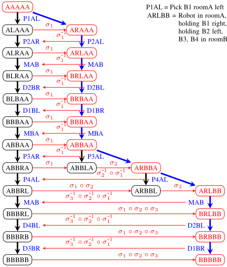
OSS explores T ′Π(S ′ , E ′ ) by A∗ and traverses an explicit search graph GOSS, which replaces any generated state s with its canonical state CΓ(s). Denoting by ρOSS(u, v) a path from u to v in GOSS, and by ρ∗OSS (s′0 , s′n ) a goal reaching path from s′0 = CΓ(s0) to a goal state s′n ∈ Ss⋆ , we call a path ρOSS in GOSS surrogate path, and a sequence of operator labels in T ′Π surrogate plan, denoted by π′ . OSSterminates search when it reaches a goal state t ∈ Ss⋆ since Γ stabilizes the goal. The final step is tracing back the optimal surrogate path ρ∗OSS (CΓ(s0), t) in the search tree TOSS to obtain a surrogate plan π′ , and tracing forward surrogate path to decode an optimal plan π from π′ . We illustrate the final decoding step for the gripper task in Figure 1.
Example 3 (TRACE-FORWARD in Gripper Task). A plan, corresponding to a black trace from the initial state, is extracted from a surrogate plan, which corresponds to a blue trace in Figure 1. These red nodes represent canonical states, while black nodes are the actual states obtained by applying the actions, when different from the canonical. Structural symmetries σ1, σ2, and σ3 are obtained from the canonical mappings and are used to map actions on the trace into an applicable sequence of actions that is a plan.
3 Orbit Space K∗ Search
In this section, we present the orbit space K∗ search algorithm (OK∗ ) for top-k planning, which alternates OSS and EA. We start by presenting a symmetry preserving singlegoal state reformulation since the earlier reformulation breaks structural symmetries. Then, we show the equivalence between plans of given planing task Π and surrogate plans reconstructed in EA, which is the basis for the soundness and completeness of OK∗ search algorithm for top-k planning. We conclude this section by highlighting the difference between K∗ and OK∗ search algorithms.
3.1 Symmetry and Single Goal State Reformulation
Some structural symmetries for the input planning task Π can disappear in a single goal state reformulated task Πg . Consider a reformulated gripper task following Katz et al. [2018b], where its single goal state sg⋆ inherits facts in an arbitrary full state in Π. It is trivial to check a structural symmetry permuting ball b1 and b2 shown in Example 2 fails to stabilize sg⋆ if {〈b1, A〉, 〈b2, B〉} ⊆ sg⋆. In order to preserve the structural symmetries of Π, we propose a new single goal state reformulation.
Proposition 1. A single goal state planning task Πg = 〈V g ,Og , sg0 , sg⋆〉 can be obtained from a planning task Π = 〈V , O, s0 , s⋆ 〉 as follows.
- V g ={v | v ∈ V} ∪ {vg}, where dom(v)=dom(v) ∪ {U} and dom(vg) = {I, U},
- sg0 = s0 ∪ {〈vg, I〉},
- sg⋆ = {〈vg, U〉} ∪ {〈v, U〉 | v ∈ V},
- Og={〈pre(o) ∪{〈vg, I〉}, eff (o)〉|o ∈ O}∪{og}, where pre(og)=s⋆ ∪ {〈vg, I〉}, eff (og)=sg⋆, and cost(og) = 0. The cost of existing actions remains the same.
Note that the additional goal-achieving zero-cost action og can be applied only once when the original goal was achieved.
No action is applicable in the new goal state, and therefore there is one-to-one correspondence between the plans of Π and those of Πg.
Theorem 1. Given a planning task Π = 〈V,O, s0 , s⋆ 〉 and the reformulated task Πg = 〈V g , Og , sg0 , sg⋆〉 shown in Proposition 1, there exists a bijective mapping between structural symmetries of Π and of Πg .
Proof. A structural symmetry σg of Πg stabilizes sg⋆ by definition, and it also stabilizes og since eff (og) = sg⋆. Thus, 〈vg, I〉 in pre(og) is mapped to itself, and so is the fact 〈vg, U〉. σg restricted to V, F , and O is a structural symmetry of Π. In the other direction, let σ be a structural symmetry of Π. We extend σ to σg of V g , F g , and Og as follows. The variable vg and its facts 〈vg, I〉 and 〈vg, U〉, as well as the action og are mapped to themselves. Each extra fact 〈v, U〉 for the variable v other than vg is mapped to 〈σ(v), U〉. It is trivial to see that σg satisfies all properties of the structural symmetries in Definition 2.
3.2 Plans in State Space and Orbit Space
OSS has shown its practical merit for cost-optimal planning [Alkhazraji et al., 2014; Sievers and Katz, 2018; Katz et al., 2018a]. The computation gain compared to A∗ stems from the fact that OSS explores a significantly smaller search space when symmetries are detected. In cost-optimal planning, or top-k planning with k=1, it is sufficient for only one optimal plan to be preserved while pruning symmetric states. For topk planning in general, however, all plans need to be preserved while pruning symmetric states.
Proposition 2. Given a planning task Π = 〈V , O, s0 , s⋆ 〉, let P denote the set of all plans in the state transition graph TΠ, and P ′ denote the set of all surrogate plans in the canonical state transition graph T ′Π relative to a structural symmetry group Γ of the planning task Π. Then, there exists a bijective mapping between plans in P and surrogate plans in P ′ .
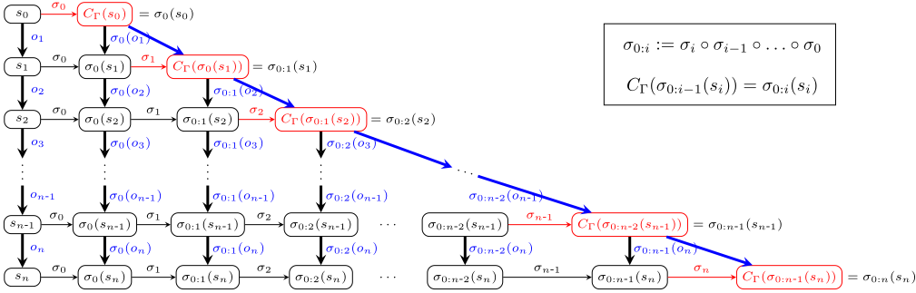
Proof. We define a bijective mapping Φ between plan traces (state action sequences) in TΠ and in T ′Π, from which the desired mapping can be straightforwardly extracted. Given a plan π=〈o1, . . . , on〉 in P that traverses a sequence of states 〈s0, s1, . . . , sn〉 over the state transition graph TΠ, let us consider a sequence φ=〈s0, o1, s1, . . . , on, sn〉, and a mapping Φ that maps φ to φ′ = 〈s′0 , o′1 , s′1 , . . . , o′n , s′n 〉 as follows.
- s′0 = CΓ(s0) and σ0 is such that σ0(s0) = CΓ(s0),
- o′1 = σ0(o1),
- s′i = CΓ(s′i-1 Jo′i K) and σi is such that σi(s′i-1 Jo′i K) = CΓ(s′i-1 Jo′i K), and
- o′i+1 = σ0:i(oi+1), where σ0:i := σi ◦ σi-1 ◦ · · · ◦ σ0.
Given that, we can also derive that s′i = σ0:i(si). Figure 2 depicts the mapping described above. The plan π and its corresponding sequence φ on the left is mapped to the sequence φ′ of red states and blue action edges, which corresponds to the surrogate plan 〈o′1 , . . . , o′n 〉. To see that φ′ corresponds to a surrogate plan, observe that (i) each state σ0:i(si) is a canonical state, (ii) the action σ0:i(oi+1) is applicable in σ0:i(si) since oi+1 is applicable in si, and (iii) applying σ0:i(oi+1)
Algorithm 1 OK∗ Search
Require: Reformulated planning task Πg , k Ensure: Top-k solution 1: Initialize OSS search 2: P ← ∅ 3: while True do 4: while ¬(OPENOSS= ∅ ∨ SWITCH-TO-EA( )) do 5: Expand an OSS node 6: PREPAREEA() 7: while ¬(OPENEA= ∅ ∨ SWITCH-TO-OSS( ) ) do 8: Expand an EA node n 9: Reconstruct surrogate plan π′ from n 10: P ← P ∪ { TRACE-FORWARD(π′ )} 11: if |P | = k then return P 12: if OPENOSS= ∅ ∧ OPENEA= ∅ then return Ptation of EA is defined relative to the canonical state transition graph T ′Πg(S ′ , E ′ ). Nevertheless, for any goal reaching surrogate path ρOSS(CΓ(sg0 ), sg⋆), the implicit path representation SIDETRACKS(ρOSS(CΓ(sg0 ), sg⋆)) still holds because GOSS is merely another digraph. Therefore, any path graph node generated by EA in orbit space can be safely reconstructed to a surrogate path, which in turn, decoded back to a plan in the state space as shown in Proposition 2.
3.4 Orbit Space K∗ Search Algorithm
Algorithm 1 shows OK∗ search algorithm for top-k planning, which takes a single goal state reformulated task Πg and k as input. Initialization steps for OSS detects structural symmetries of Πg and creates necessary data structure to explore the canonical state transition graph T ′Πg (line 1). After initializing P to store found plans (line 2), OK∗ alternates OSS (line 4-5) and EA (line 7-11). OSS explores T ′Πg until it exhausts the search space or SWITCH-TO-EA() triggers to stop expanding nodes in OSS. The latter happens when either the lowest f value in the OSS queue is no smaller than the one in the EA queue, or a pre-defined threshold on the number of expanded nodes since previous switch is reached. Before initiating EA, PREPAREEA() builds necessary data structures
in σ0:i(si) results in a state σ0:i(siJoi+1K) = σ0:i(si+1), whose canonical state is σ0:i+1(si+1). Finally, since sn is a goal state, so is s′n = σ0:n(sn). We show now that Φ is injective. For sequences φ1 = 〈s10 , o11 , s11 , . . . , o1n , s1n 〉 and φ2 = 〈s20 , o21 , s21 , . . . , o2n , s2n 〉 with s10 = s20 = s0, if Φ(φ1) = Φ(φ2), then we show by induction that the two sequences must be equivalent. Note that Φ(φ1 ) can be written as 〈σ1 0 (s0), σ1 0 (o11 ), σ1 0:1 (s11 ), . . . , σ1 0:n-1 (o1n ), σ1 0:n (sn)〉, and Φ(φ2 ) in a similar way. Base: s10 = s20 = s0 and σ1 0 (s0) = σ2 0 (s0) = CΓ(s0). Therefore σ1 0 = σ2 0 . Step: if s1i = s2i and σ1 i = σ2 i for i ≤ m, we show that o1m+1 = o2m+1 and s1m+1 = s2m+1 . From the equivalence of Φ(φ1 ) and Φ(φ2 ), we have σ1 0:m(o1m+1 ) = σ2 0:m(o2m+1 ). Since σ1 0:m = σ2 0:m, we must have o1m+1 = o2m+1 . Since φ1 and φ2 correspond to plans, we have s1m+1 = s1mJo1m+1 K and s2m+1 = s2mJo2m+1 K, giving us s1m+1 = s2m+1 .
We conclude by showing that Φ is surjective. For a surrogate plan π′ = 〈o′1 , . . . , o′m〉 and its corresponding sequence φ′ = 〈s′0 , o′1 , s′1 , . . . , o′n , s′n 〉, we have s′0 = CΓ(s0) and s′i = CΓ(s′i-1 Jo′i K). Let σ0 be such that σ0(s0) = s′0 = CΓ(s0) and for 1 ≤ i ≤ n, let σi be such that σi(s′i-1 Jo′i K) = s′i . Let oi = σ-1 0:i-1 (o′i ) be the actions that are obtained by applying the inverse of the structural symmetry σ0:i-1 to o′i . We show that π = 〈o1, . . . , on〉 is a plan and for its corresponding sequence φ we have Φ(φ) = φ′ . Let si = σ-1 0:i (s′i ). First, observe that s0 = σ-1 0 (s′0 ). We need to show that (i) oi is applicable in si-1 and (ii) applying oi in si-1 results in si. For (i) we know that o′i is applicable in s′i-1 and for any σ ∈ Γ, σ(o′i ) is applicable in σ(s′i-1 ), and in particular for σ-1 0:i-1 . For (ii), s′i = σi(s′i-1 Jo′i K) and therefore σ-1 i (s′i ) = s′i-1 Jo′i K. Now, si-1JoiK = σ-1 0:i-1 (s′i-1 )Jσ-1 0:i-1 (o′i )K = σ-1 0:i-1 (s′i-1 Jo′i K) = σ-1 0:i-1 (σ-1 i (s′i )) = σ-1 0:i (s′i ) = si.
3.3 Implicit Path Representation in Orbit Space
Given a single goal state reformulated planning task Πg = 〈V g , Og , sg0 , sg⋆〉, EA in K∗ builds path graph P(GA∗) from an explicit search graph GA∗ of A∗ by exploring TΠg (S, E). When EA traverses a path graph P(GOSS) derived from an explicit search graph GOSS of OSS, the implicit path represensuch as OPENEA and heap graphs [Eppstein, 1998]. EA traverses the path graph of the sub-graph of T ′Πg developed by OSS. For a path graph node, OK∗ first reconstructs surrogate plan π′ , and then decodes it to a plan π by TRACE-FORWARD [Domshlak et al., 2015]. If the lowest f value in the OSS queue is smaller than the one in the EA queue, SWITCH-TO-OSS() triggers, forcing a switch back to OSS. All the changes from the K∗ algorithm are marked in blue. OK∗ terminates either when it finds top-k plans for a solvable top-k problem (line 11) or it exhausts both open lists before finding k plans for an unsolvable top-k problem (line 12).
| LMcut | M&S | CEGAR | iPDB | BLIND | ||||||||||
|---|---|---|---|---|---|---|---|---|---|---|---|---|---|---|
| SymK | FI | K∗ | OK∗ | (+)K∗ | K∗ | OK∗ | K∗ | OK∗ | K∗ | OK∗ | K∗ | OK∗ | ||
| SymK | 0 | 36 | 27 | 20 | 33 | 34 | 28 | 36 | 31 | 30 | 25 | 46 | 37 | |
| FI | 20 | 0 | 19 | 6 | 29 | 30 | 23 | 27 | 20 | 21 | 14 | 31 | 26 | |
| K∗ | 26 | 37 | 0 | 1 | 32 | 34 | 28 | 30 | 30 | 17 | 15 | 46 | 40 | |
| LMcut OK∗ | 32 | 45 | 30 | 0 | 45 | 47 | 35 | 45 | 36 | 30 | 19 | 57 | 50 | |
| (+)K∗ | 17 | 29 | 15 | 8 | 0 | 6 | 2 | 25 | 16 | 11 | 8 | 41 | 29 | |
| M&S K∗ | 17 | 30 | 12 | 6 | 2 | 0 | 0 | 22 | 12 | 7 | 5 | 41 | 27 | |
| OK∗ | 20 | 34 | 23 | 12 | 22 | 24 | 0 | 31 | 23 | 20 | 9 | 48 | 41 | |
| K∗ | 19 | 31 | 11 | 9 | 20 | 22 | 20 | 0 | 8 | 10 | 10 | 39 | 28 | |
| CEGAR OK∗ | 23 | 34 | 22 | 10 | 30 | 32 | 22 | 25 | 0 | 23 | 9 | 48 | 33 | |
| K∗ | 30 | 38 | 22 | 19 | 35 | 36 | 32 | 32 | 28 | 0 | 1 | 48 | 38 | |
| iPDB OK∗ | 34 | 41 | 33 | 25 | 44 | 47 | 35 | 41 | 36 | 22 | 0 | 54 | 46 | |
| K∗ | 11 | 28 | 3 | 1 | 7 | 7 | 7 | 2 | 1 | 3 | 2 | 0 | 0 | |
| BLIND OK∗ | 15 | 31 | 14 | 3 | 17 | 17 | 7 | 19 | 2 | 12 | 2 | 29 | 0 | |
| Overall Coverage | 892 | 652 | 933 | 1022 | 786 | 769 | 834 | 803 | 868 | 862 | 932 | 587 | 695 | |
Theorem 2. Algorithm 1 (OK∗ ) is sound and complete for top-k planning.
Proof. Let Π be a planning task and let P ⊆ PΠ be the set of plans found by Algorithm 1 for k. We show that P is a solution to top-k planning problem. First, if |P| < k, then the algorithm terminated in line 12. Thus, it has exhausted the orbit space and reconstructed plans that correspond to all surrogate plans in the orbit space. From Proposition 2 we have an isomorphism between the (finite) set of surrogate plans in the orbit space and PΠ, the set of plans of Π. Therefore, we must have P = PΠ.
Now, suppose the algorithm terminated in line 11 and let ρ′ be the surrogate path extracted last before the termination. Then for all π ∈ P, we have cost(π) ≤ cost(ρ′ ), since EA nodes are expanded in the order of their costs. Assume to the contrary that there exists a plan π ̸∈ P, such that cost(π) < cost(π′ ) for some π′ ∈ P. Then, according to Proposition 2, let ρ be the surrogate plan that corresponds to π. Since π ̸∈ P , EA did not expand the node that corresponds to ρ yet. However, note that we have cost(ρ) < cost(ρ′ ), contradicting the expansion order of EA.
4 Experimental Evaluation
To empirically evaluate the effectiveness of using structural symmetries with K∗ , we have implemented our suggested algorithm OK∗ on top of an existing K∗ implementation
[Lee et al., 2023] within the Fast Downward planning system [Helmert, 2006]. All experiments were performed on Intel(R) Xeon(R) Gold 6248 CPU @ 2.50GHz machines, with the timeout of 30 minutes and memory limit of 8GB per run. The benchmark set consists of all benchmarks from optimal tracks of International Planning Competitions 1998-2018, a total of 1827 tasks in 65 domains. We have experimented with four admissible heuristics, LMcut [Helmert and Domshlak, 2009], merge-and-shrink abstraction (denoted by M&S) [Helmert et al., 2007], counterexample-guided Cartesian abstraction refinement (denoted by CEGAR) [Seipp and Helmert, 2018], and pattern database heuristic iPDB [Haslum et al., 2007], as well as with the blind heuristic. We measure the total time for finding the top-k solution for a given k, as well as the coverage: 1 per task if the top-k solution was found, 0 otherwise. In addition to comparing OK∗ to K∗ with the aforementioned heuristics, we compare to the planners that implement the other two approaches to top-k planning, bi-directional symbolic search (SymK) [Speck et al., 2020] and Forbid Iterative (FI) [Katz et al., 2018b]. Following previous work, all planners are using the same translator and no additional preprocessing, as the preprocessing can remove some actions that could otherwise be part of valid plans. The merge-and-shrink abstraction performs an optimization, pruning abstract states that are unreachable from the (abstract) initial state. This optimization must be turned off when using orbit space search. In our experiments, we compare to both with and without the optimization when using K∗ . To differentiate the two, we mark the configuration with the optimization by (+) .
Table 1 shows the pairwise comparison of the tested approaches for k = 1000. Each entry denotes the number of domains where the row planner achieves a better summed coverage than the column planner. Additionally, the last row denotes the overall coverage for each planner. The winners are marked in bold. For the pairwise comparison, the value in (x,y) is bolded if it is larger than the value in (y,x), that is planner x excelled over planner y in more domains than planner y excelled over planner x. First, note that there are a few instances solved by K∗ but not by OK∗ , specifically 25 for the CEGAR heuristic and one for each of the other heuristic. While a few of these instances are due to minor time fluctuations, the rest appear to be due to (abstraction based) heuristics not being as informative on canonical states as on states reachable from the initial state. Despite that shortcoming, we observe that OK∗ consistently significantly outperforms K∗ . The largest overall coverage increase occurs for the blind heuristic, 108 tasks. Next is LMcut with 89 tasks, iPDB with 70 tasks, and CEGAR and M&S with 65 tasks each. The best performing overall configuration is OK∗ with LMcut heuristic, passing SymK by 130 tasks overall. Looking at domain level performance, LMcut wins over SymK in 32 domains and loses in 20, showing superior performance. Comparing to other configurations on a domain level coverage, LMcut almost always wins in more domains than it loses in. The only exception is OK∗ with iPDB, which is the best domain level performer, always winning in more domains than it is losing in and winning over LMcut in 25 domains, loosing in 19.
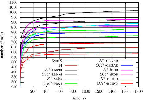
As many planning applications might require a shorter planning time, we test the any-time performance of OK∗ compared to the other approaches. The results for top-k coverage for k = 1000 as a function of time are depicted in Figure 3. The lines for the same heuristic are depicted with the same color, solid line for OK∗ and dashed line for K∗ . Our first observation is that for all heuristics and all timeouts, the configurations that run OK∗ significantly outperform the K∗ configurations. The overall best performer for almost all tested timeouts is OK∗ with LMcut heuristic. Only between 100 and 150 seconds it loses the first place to OK∗ with iPDB. For these timeouts, the difference in overall coverage between the two approaches peaks at 6 tasks. Somewhat surprisingly, for small timeouts of up to 45 seconds, the second best is K∗ with LMcut. From 50 seconds to 1700 seconds, OK∗ with iPDB is the second best. From 1700 till 1760 it is tied with K∗ with LMcut, which takes the lead for the last 40 seconds. It is worth mentioning that OK∗ with iPDB achieves almost its maximal coverage (922 out of 932) and levels out in under 400 seconds. The coverage of OK∗ with LMcut, on the other hand, keeps rising up with more allocated time.
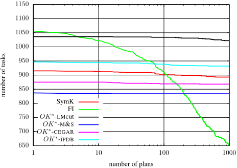
Finally, to test the performance of our approach for smaller k values, Figure 4 depicts the top-k coverage as a function of k. Note here that for very small values of k, FI still outperforms all other approaches. For k = 1, as in cost-optimal planning, FI achieves the overall coverage of 1056 vs. 1036 for OK∗ with LMcut. Since FI uses internally OSS with LMcut and partial order reduction, and OK∗ for k = 1 is essentially equivalent to OSS, the difference stems from our methods not being able yet to benefit from partial order reduction. As FI needs to iteratively run a cost-optimal planner, it quickly loses its benefit and OK∗ with LMcut takes the lead already for k = 5 and keeps the first place for all k ≥ 5. FI keeps the second place until k = 72, where OK∗ with iPDB catches up, keeping the second place from that point onward. SymK takes the third place starting from k = 107. It is worth noting that OK∗ configurations (as well as SymK and K∗ ) do not lose much coverage when going to larger k values, allowing to generate many plans quickly.
5 Conclusions and FutureWork
In this work, we exploit structural symmetries to improve the performance of K∗ search. For that, we propose a new singlegoal planning task transformation that preserves the symmetries of the input task. We formally prove a property of the orbit space that allows us to apply K∗ to it. We show that the proposed algorithm is sound and complete for top-k planning and perform an experimental evaluation that establishes our approach as the new state of the art for top-k planning.
In the future work we intend to further improve OK∗ for top-k planning by integrating another pruning technique, partial order reduction [Wehrle and Helmert, 2012]. In contrast to symmetry based pruning, applying partial order reduction does prune some of the goal paths in the search space [Katz and Lee, 2023], and therefore great care must be taken to ensure that all plans can be found. Another promising direction is integrating symmetries explicitly into Eppstein's algorithm, to reduce both the computational effort and the memory consumption required for storing all paths by storing symmetric paths within the same node.
@inproceedings{ijcai2023p596,
  title     = {K∗ Search over Orbit Space for Top-k Planning},
  author    = {Katz, Michael and Lee, Junkyu},
  booktitle = {Proceedings of the Thirty-Second International Joint Conference on
               Artificial Intelligence, {IJCAI-23}},
  publisher = {International Joint Conferences on Artificial Intelligence Organization},
  editor    = {Edith Elkind},
  pages     = {5368--5376},
  year      = {2023},
  month     = {8},
  note      = {Main Track},
  doi       = {10.24963/ijcai.2023/596},
  url       = {https://doi.org/10.24963/ijcai.2023/596},
}
TY - CPAPER TI - K∗ Search over Orbit Space for Top-k Planning AU - Katz, Michael AU - Lee, Junkyu T2 - Proceedings of the Thirty-Second International Joint Conference on Artificial Intelligence, IJCAI-23 PB - International Joint Conferences on Artificial Intelligence Organization PY - 2023 SP - 5368 EP - 5376 DO - 10.24963/ijcai.2023/596 UR - https://doi.org/10.24963/ijcai.2023/596 ER -Copied
Machine-readable versions of this paper, for tools and AI agents:





