
Mean Payoff Optimization for Systems of Periodic Service and Maintenance
Proceedings of the Thirty-Second International Joint Conference on Artificial Intelligence. Main Track. Pages 5386-5393.
https://doi.org/10.24963/ijcai.2023/598
Keywords
- Planning and Scheduling: PS: Routing
- Robotics: ROB: Motion and path planning
- Planning and Scheduling: PS: Robot planning
Abstract
Consider oriented graph nodes requiring periodic visits by a service agent. The agent moves among the nodes and receives a payoff for each completed service task, depending on the time elapsed since the previous visit to a node. We consider the problem of finding a suitable schedule for the agent to maximize its long-run average payoff per time unit. We show that the problem of constructing an epsilon-optimal schedule is PSPACE-hard for every fixed non-negative epsilon, and that there exists an optimal periodic schedule of exponential length. We propose randomized finite-memory (RFM) schedules as a compact description of the agent's strategies and design an efficient algorithm for constructing RFM schedules. Furthermore, we construct deterministic periodic schedules by sampling from RFM schedules.
- [Basilico et al., 2009] N. Basilico, N. Gatti, and F. Amigoni. Leader-follower strategies for robotic patrolling in envi- ronments with arbitrary topologies. In Proceedings of AA- MAS 2009, pages 57-64, 2009.
- [Bertels and Fahle, 2006] S. Bertels and T. Fahle. A hybrid setup for a hybrid scenario: Combining heuristics for the home health care problem. Computers & Operations Re- search, 33(10):2866-2890, 2006.
- [Bostel et al., 2008] N. Bostel, P. Dejax, P. Guez, and F. Tri- coire. Multiperiod planning and routing on a rolling hori- zon for field force optimization logistics. In The Vehicle Routing Problem: Latest Advances and New Challenges. Springer, 2008.
- [Boussier et al., 2007] S. Boussier, D. Feillet, and M. Gen- dreau. An exact algorithm for team orienteering problems. 4OR-Q J. Oper. Res., 5:211-230, 2007.
- [Castillo-Salazar et al., 2016] J. Arturo Castillo-Salazar, Dario Landa-Silva, and Rong Qu. Workforce scheduling and routing problems: Literature survey and computa- tional study. Ann. Oper. Res., 239:39-67, 2016.
- [Chen et al., 2016] Y. Chen, F. Polack, P. Cowling, P. Mour- djis, and S. Remde. Risk driven analysis of mainte- nance for a large-scale drainage system. In Proceedings of ICORES 2016, pages 296-303. SciTePress, 2016.
- [Cordeau et al., 2010] J.-F. Cordeau, G. Laporte, F. Pasin, and S. Ropke. Scheduling technicians and tasks in a telecommunications company. Journal of Scheduling, 13(4):393-409, 2010.
- [Dahite et al., 2020] L. Dahite, A. Kadrani, R. Benmansour, R.N. Guibadj, and C. Fonlupt. Optimization of mainte- nance planning and routing problems. In R. Benmansour, A. Sifaleras, and N. Mladenović, editors, Variable Neigh- borhood Search. Springer, 2020.
- [Ehrenfeucht and Mycielski, 1979] A. Ehrenfeucht and J. Mycielski. Positional strategies for mean payoff games. International Journal of Game Theory, 8:109-113, 1979.
- [Eveborn et al., 2006] P. Eveborn, P. Flisberg, and M. Rönnqvist. Laps Care -an operational system for staff planning of home care. European Journal of Operational Research, 171(3):962-976, 2006.
- [Ho and Ouaknine, 2015] Hsi-Ming Ho and J. Ouaknine. The cyclic-routing UAV problem is PSPACE-complete. In Proceedings of FoSSaCS 2015, volume 9034 of LNCS, pages 328-342. Springer, 2015.
- [Jbili et al., 2018] S. Jbili, A. Chelbi, M. Radhoui, and M. Kessentini. Integrated strategy of vehicle routing and maintenance. Reliab. Eng. Syst. Saf., 170:202-214, 2018.
- [Kallehauge et al., 2005] B. Kallehauge, J. Larsen, O.B. Madsen, and M.M. Solomon. Vehicle routing problem with time windows. In Column Generation. Springer.
- [Kingma and Ba, 2015] D. P. Kingma and Jimmy Ba. Adam: A method for stochastic optimization. In Proceedings of ICLR 2015, 2015.
- [Klaška et al., 2021] D. Klaška, A. Kučera, V. Musil, and V. Řehák. Regstar: Efficient strategy synthesis for adver- sarial patrolling games. In Proceedings of UAI 2021, pages 471-481, 2021.
- [Klaška et al., 2023] D. Klaška, A. Kučera, V. Musil, and V. Řehák. Mean Payoff Optimization for Systems of Periodic Service and Maintenance. arXiv:2305.08555 [cs.GT], 2023.
- [Kovacs et al., 2011] A.A. Kovacs, S.N. Parragh, K.F. Do- erner, and R.F. Hartl. Adaptive large neighborhood search for service technician routing and scheduling problems. Journal of Scheduling, 15(5):579-600, 2011.
- [López-Santana et al., 2016] E. López-Santana, R. Akhavan-Tabatabaei, L. Dieulle, N. Labadie, and A.L. Medaglia. On the combined maintenance and routing optimization problem. Reliab. Eng. Syst. Saf., 145:199-214, 2016.
- [Norris, 1998] J.R. Norris. Markov Chains. Cambridge Uni- versity Press, 1998.
- [Paszke et al., 2019] A. Paszke, S. Gross, F. Massa, A. Lerer, J. Bradbury, G. Chanan, T. Killeen, Z. Lin, N. Gimelshein, L. Antiga, A. Desmaison, A. Kopf, E. Yang, Z. DeVito, M. Raison, A. Tejani, S. Chilamkurthy, B. Steiner, Lu Fang, J. Bai, and S. Chintala. Pytorch: An imperative style, high- performance deep learning library. In Advances in Neu- ral Information Processing Systems 32, pages 8024-8035.
- Curran Associates, Inc., 2019.
- [Pillac et al., 2013] V. Pillac, C. Guéret, and A.L. Medaglia. A parallel matheuristic for the technician routing and scheduling problem. Optim. Lett., 7:1525-1535, 2013.
- [Souffriau et al., 2013] W. Souffriau, P. Vansteenwegen, G. Vanden Berghe, and D. Van Oudheusden. The mul- ticonstraint team orienteering problem with multiple time windows. Transportation Science, 47(1):53-63, 2013.
- [Tang et al., 2007] H. Tang, E. Miller-Hooks, and R. Tomas- tik. Scheduling technicians for planned maintenance of geographically distributed equipment. Transportation Research Part E: Logistics and Transportation Review, 43(5):591-609, 2007.
- [Tarjan, 1972] R. Tarjan. Depth-first search and linear graph algorithms. SIAM Journal of Computing, 1(2), 1972.
- [Toth and Vigo, 2001] P. Toth and D. Vigo. The Vehicle Routing Problem. SIAM Monographs on Discrete Mathe- matics and Applications. SIAM, 2001.
- [Vorobeychik et al., 2012] Y. Vorobeychik, B. An, and M. Tambe. Adversarial patrolling games. In Proceedings of AAAI 2012, pages 91-98, 2012.
- [Xu and Chiu, 2001] J. Xu and S.Y. Chiu. Effective heuris- tic procedures for a field technician scheduling problem. Journal of Heuristics, 7:495-509, 2001.
- [Zamorano and Stolletz, 2017] E. Zamorano and R. Stolletz. Branch-and-price approaches for the Multiperiod Techni- cian Routing and Scheduling Problem. European Journal of Operational Research, 257(1):55-68, 2017.
References were extracted automatically from the PDF and may contain errors.
Full text extracted automatically from the PDF; figures, tables and equations may differ. The PDF is the version of record.
1 Introduction
Workforce scheduling and routing problems (WSRP) [Castillo-Salazar et al., 2016] refer to scenarios involving mobile personnel performing periodic service or maintenance at different locations, where the transport time significantly influences the overall efficiency. Hence, WSRP is a combination of employee scheduling and vehicle routing problems (VRP) [Toth and Vigo, 2001], where the latter provides the methodology for computing appropriate trajectories for service agents. Since services can be performed at customers' locations only in certain time intervals, the vehicle routing problem with time windows (VRPTW) [Kallehauge et al., 2005] is particularly relevant in this setting.
An instance of VRPTW is a finite set of nodes S where each v ∈ S is assigned a time interval [av, bv]. A vehicle must arrive to v before time bv, and if it arrives before time av, it must wait until av. Moving between v, u takes time time( ), and costs c(v, u). The task is to design a set of routes for a given number of vehicles minimizing the total costs such that each node is visited precisely once and on time. The routes are obliged to start/end at designated nodes (depots), and there is a time horizon b bounding the length of every route such that bv ≤ b for every v. Intuitively, the b corresponds to one working shift.
1.1 Motivation
Although VRPTW is appropriate for modeling the "routing component" of many periodic maintenance problems, it is not applicable in situations when the maintenance period demanded by a customer is significantly larger than one working shift, and the preference for the period is specified by a non-trivial payoff function rather than just lower/upper bounds. To understand the need to overcome these limitations, consider the following simple scenario.
Let S be a set of public vending machines requiring periodic maintenance. For each machine v, let rv be the time after which v needs another preventive service action. Note that rv may range from days to weeks. The owner of the machines demands a maintenance period rv for every v and is willing to pay pv for each service action, i.e. spend pv rv per time unit for maintenance costs. If v is serviced prematurely at time t < rv, the owner has no reason to complain, but it insists on keeping the same maintenance costs per time unit, i.e., the agent receives only t · pv rv for this service. If v is serviced at time t > rv, the owner charges a negative penalty cv < 0 for every time unit exceeding rv, i.e., the agent receives pv + (t - rv) · cv. The owner may also introduce extra penalties for very short times. The aim of the agent is to maximize the average payoff per time unit. To avoid costly premature returns to certain nodes, the agent may prolong the actual traversal time between two nodes by non-negative waits.
Note that the above scenario does not impose any bounded planning horizon. The agent may still be required to return to a depot after b time units (a working shift), which can be modelled by a node where significant deviations from b are "punished" by a negative payoff. Also, note that the payoff function can be even more complicated in scenarios where the timing constraints are influenced by multiple criteria.
1.2 Our Contribution
We introduce and study the infinite horizon recurrent routing problem (IHRRP) specified as a tuple S = (S, time, {Pv : v ∈ S},D) where S is a finite set of nodes, time(v, u) is the traversal time between the nodes v and u, Pv(t) is a payoff received by a service agent when v is revisited after exactly t time units, and D ⊆ S × S is a subset of moves along which the agent is allowed to wait. The problem is to compute an appropriate schedule (moving plan) for the agent maximizing the mean payoff, i.e. the long-run average payoff per time unit. Our main results (1)-(4) are summarized below.
- We show (Theorem 1) that for every ε ≥ 0, there exists an ε-optimal schedule which is deterministic and periodic. Such a schedule can be represented as a finite cycle over the nodes, and the length of this cycle is at most singly exponential in size of S .
- We prove (Theorem 2) that solving IHRRP is PSPACEhard, even when demanding only sub-optimal solutions. More precisely, it is PSPACE-hard to distinguish whether the best mean payoff achievable for a given instance S is at least 1 or at most 1-ε for arbitrary ε ≥ 0.
According to (2), the optimal achievable mean payoff is not only hard to compute but also hard to approximate up to an arbitrary fixed ε ≥ 0. Hence, there is no efficient algorithm for constructing an ε-optimal schedule (randomized or deterministic), assuming P ̸= PSPACE. Furthermore, (2) implies that the length of a cycle representing an ε-optimal deterministic and periodic schedule of (1) cannot be bounded by any polynomial, unless NP = PSPACE. Hence, the exponential upper bound on its length established in (1) is matched by the superpolynomial lower bound.
In principle, the upper bound of (1) allows for constructing an ε-optimal deterministic schedule by the methods invented for finite-horizon routing problems. These methods are mostly based on solving appropriate mathematical programs whose size is proportional to the horizon, and a solution is computable in NP. Since we need to consider an exponentially large horizon for IHRRP, the size of these programs becomes exponential, making the total running time even doubly exponential. This explains why the techniques for finite-horizon routing problems are not applicable to the infinite-horizon case. In this work, we use a different algorithmic approach.
- We introduce the concept of randomized finite-memory (RFM) schedules and design a polynomial-time algorithm for constructing a RFM schedule for a given IHRRP instance based on differentiable programming and gradient ascent (Algorithm 1).
Finite-memory strategies are equipped with a finite set M of memory states. In each step, the agent's (possibly randomized) decision depends on its current location v ∈ S and its current memory state m ∈ M. Intuitively, the memory states are used to "remember" some finite information about the sequence of previous moves executed by the agent. In general, an ε-optimal RFM schedule may require memory with exponentially many states. However, randomization helps to reduce this blowup. RFM schedules can achieve a substantially higher mean payoff than deterministic schedules with the same (or even larger) memory. This is the crucial tool for tackling the PSPACE-hardness of the IHRRP problem.
Randomized schedules are easily executable by robotic devices, but they are less appropriate for human agents 1 . Therefore, we also consider the problem of constructing a deterministic schedule.
1 Previous works on finite horizon routing problems consider only deterministic strategies.
- We design an algorithm for constructing a deterministic periodic schedule for a given IHRRP instance based on identifying optimal cycles in long routes generated by a previously computed RFM schedule (Algorithm 2).
The routes are obtained by repeatedly "executing" a constructed RFM schedule. As we shall see in Section 4.2, RFM schedules are ergodic, and the probability that a route of length n contains a cycle achieving the same or even better mean payoff as the considered RFM schedule converges to one as n approaches infinity.
The algorithms of (3) and (4) are evaluated on instances of increasing size. We use planar grids with randomly positioned nodes to avoid bias towards simple instances. The algorithms process relatively large instances and produce highquality schedules. The quality of cycles discovered by the algorithm of (4) grows with the quality of RFM schedules used to generate long routes. The length of the resulting cycles exceeds 12 working shifts, and the corresponding mean payoff is not achievable by short cycles corresponding to one shift (a typical planning horizon in finite-horizon routing problems).
1.3 Example
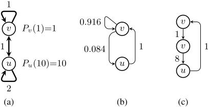
To get some intuition about our results, consider an instance S of Fig. 1 (a) with two nodes v, u. The traversal times are indicated by transition labels. The payoff functions Pv, Pu satisfy Pv(t) = 1 for all t ≥ 1, and Pu(t) is either 10 or 0 depending on whether t ≥ 10 or not, respectively. The agent can wait along all transitions.
A simple RFM schedule is shown in Fig 1 (b). As |M| = 1, this schedule corresponds to a positional (Markovian) strategy. For example, whenever the agent visits v, it either performs a self-loop on v or moves to u with probability 0.916 and 0.084, respectively. This trivial RFM schedule achieves a mean payoff 1.307. The best deterministic schedule with |M| = 1 performs the self-loop on v forever, and the associated mean payoff is 1. A deterministic schedule with |M| = 2 can achieve a mean payoff equal to 1.1 in the way shown in Fig 1 (c). The schedule performs one self-loop on v, then moves to u (prolonging the traversal time to 8 by waiting), and then returns back to v. This cycle is repeated forever. Note that two memory states are needed to "remember" whether the self-loop on v has already been performed or not.
In fact, a deterministic schedule needs |M| ≥ 4 to achieve a mean payoff better than 1.307. Hence, even in this trivial example, using randomization with |M| = 1 achieves better mean payoff than deterministic schedules with |M| = 3, illustrating the advantage of RFM schedules mentioned above.
Now, let us consider the algorithm of (4) when the constructed RFM schedule with |M| = 1 is used to generate long routes in the considered instance. Due to the large probability of the self-loop on v, a randomly generated route initiated in v tends to start with "many" copies of v eventually followed by u. Hence, the optimal deterministic and periodic schedule with mean payoff 1.9 represented by the cycle v, 1, v, 1, v, 1, v, 1, v, 1, v, 1, v, 1, v, 1, v, 1, u, 1, v is discovered quickly. This illustrates how the constructed RFM schedule "navigates" the search for a cycle with high mean payoff.
1.4 RelatedWork
Most of the existing works dealing with routing and maintenance optimization use the routing model to plan maintenance operations and thus divide the optimization task into two phases. Examples include the Technician Routing and Scheduling Problem [Zamorano and Stolletz, 2017], the Technician and Task Scheduling Problem [Cordeau et al., 2010], the Service Technician Routing and Scheduling Problem [Kovacs et al., 2011], or the Geographically Distributed Asset Maintenance Problem [Chen et al., 2016]. More recent works [L´opez-Santana et al., 2016; Jbili et al., 2018] combine maintenance and routing models into one optimization framework. We refer to [Castillo-Salazar et al., 2016; Dahite et al., 2020] for more detailed overviews.
The above models are finite-horizon, and the existing solution approaches can be classified as (i) heuristics and metaheuristics, (ii) mathematical programming, (iii) hybrid methods. Examples of heuristic methods are local search [Souffriau et al., 2013], adaptive large neighborhood search [Kovacs et al., 2011; Cordeau et al., 2010; Pillac et al., 2013], tabu search [Tang et al., 2007], greedy heuristics [Xu and Chiu, 2001], etc. Mathematical programming approaches are mostly based on constructing a mixed integer program and then applying commercial solvers or using branch-and-price or similar algorithms (e.g., [Bostel et al., 2008; Boussier et al., 2007]). Hybrid approaches are based, e.g., on the combination of linear programming, constraint programming, and metaheuristics [Bertels and Fahle, 2006], or the combination of linear programming and repeating matching heuristics [Eveborn et al., 2006]. A more comprehensive overview can be found in [Zamorano and Stolletz, 2017].
Randomized strategies for infinite horizon path planning problems have been used in the context of adversarial patrolling [Vorobeychik et al., 2012; Basilico et al., 2009; Klaˇska et al., 2021]. Here, randomization is crucial for decreasing the predictability of the patroller. Technically, the patrolling problem is a variant of recurrent bounded reachability optimization which is different from the considered IHRRP problem.
To the best of our knowledge, infinite horizon routing problems related to periodic maintenance have not yet been studied in previous works.
2 Mathematical Model
We use N and N+ to denote the sets of all non-negative and positive integers, respectively. We assume familiarity with basic notions of probability theory and Markov chain theory (ergodicity, invariant distribution, etc.).
2.1 Service Specification
Let S be a finite set of nodes, and let time : S × S → N+ be a function such that time(v, u) is the time needed to move from v to u. Performing a service action at a node v also takes some time, but we assume that this time has already been added to time(v, u) for every u. This also explains why time(v, v) can be positive.
For every v ∈ S, let Pv : N+ → R be a function such that Pv(t) is the payoff received by a service agent when v is
1
revisited after time t units. We require that Pv is eventually affine, i.e., there exist kv ∈ N+ and dv, cv ∈ R such that Pv(kv+t) = dv +t · cv for all t ∈ N. Note that no restrictions are imposed on the values of Pv(t) for t < kv.
The constant kv is typically chosen sufficiently large so that revisiting v after more than kv time units is highly undesirable and f(kv+i) is negative for all i ≥ 0. Then, the agent is not motivated to re-visit v after kv time units, and hence the precise value of f(kv+i) does not matter. The exact purpose of the constant cv is clarified in Section 2.2 (it is used to prevent the agent from suspending visits to a certain subset of nodes).
When an agent moves between v and u, it may intentionally prolong the traversal time beyond time(v, u) if this leads to a higher payoff. Since the underlying transport infrastructure may allow for prolonging only certain moves, we specify a subset D ⊆ S × S of prolongable moves.
A service specification is defined as a tuple S = (S, time, {Pv : v ∈ S},D). Every Pv is represented as a finite sequence Pv(1), . . . , Pv(kv), dv, cv, where all numbers are written in binary. The enconding size of S , denoted by ||S||, is the length of the (binary) string representing S. We also use kmax to denote max{kv : v ∈ S}.
Remark 1. Our model of service specification is intentionally simplified so that all optimization criteria except for return times are eliminated, allowing for studying the "timing aspects" of the IHRRP problem in isolation. Additional features, such as costs associated to moves, waits, service actions, etc., are straightforward extensions resulting in more technical (but not substantially different) variant of the objective function governing the algorithm presented in Section 5.
2.2 General Deterministic Schedules, Mean Payoff
A deterministic schedule (or just a schedule) is an infinite sequence α = v1, τ1, v2, τ2, v3, τ3, . . . where vi ∈ S and τi = time(vi, vi+1)+wi is the time spent by moving from vi to vi+1. Here, wi ≥ 0 is an integer wait prolonging the move. We require that wi > 0 only if (vi, vi+1) ∈ D.
Every schedule α determines the associated mean payoff MP(α), defined as the long-run average payoff per time unit. For every i ≥ 1, let ℓi be the index of the previous visit to vi (if there is no previous visit to vi, then ℓi = 1). We also use ti to denote the total time elapsed since the previous visit to vi, i.e. ti = ∑i-1 j=ℓi τj. Nowwe define
Clearly, MP(α) = MP(α′ ) for every infinite suffix α′ of α.
In general, a schedule may avoid servicing some nodes and visit only a convenient subset of S generating a high mean payoff. However, in some cases, the agent may be required to service a certain subset C ⊆ S of compulsory nodes (such as the node modeling the depot, see Section 1). We implement this requirement as a soft constraint in the sense that the agent may still avoid visiting v ∈ C if it is willing to pay the penalty cv per every time unit. If cv is set to a sufficiently negative value, then omitting v results in a negative mean payoff. Hence, the synthesis algorithm aims to avoid this situation by revisiting v infinitely often. In some instances, setting the penalty cv to a "moderately negative" value makes sense. For example, suppose the agent can hire an external provider for servicing v. In that case, the penalty cv may represent the long-run average costs generated by this subcontract, and suspending visits to a compulsory v may be an eligible rational decision for the agent. For technical convenience, from now on we assume that cv = 0 for all v ̸∈ C.
For every schedule α = v1, τ1, v2, τ2, v3, τ3, . . ., let F(α) be the set of all v ∈ S that occur only finitely often in α (i.e. v = vi for finitely many i ∈ N+). We put
In other words, MPC (α) is the long-run average payoff per time unit when the agent commits to α and the set of compulsory nodes is C. It may happen that MPC (α) is negative, which means that the agent is losing money in the long run and it should better not follow the schedule α. Furthermore, we define
For a given ε ≥ 0, we say that α is ε-optimal if ValC -MPC (α) ≤ ε. In particular, 0-optimal schedules are called optimal.
3 Deterministic Periodic Schedules
General schedules are not finitely representable and hence not apt for algorithmic purposes. A workable subclass of deterministic schedules are periodic schedules. A schedule α is periodic if there exists a finite generating cycle β = v1, τ1, . . . , vn such that v1 = vn and α is the concatenation 2 of infinitely many copies of β, i.e., α = β ⊙ β ⊙ · · · . The length of β is defined as n - 1.
Now we precisely formulate and prove the results (1) and (2) presented in Section 1. Since the proofs are not strictly needed for understanding the meaning and consequences of our theorems, they are given in the extended version of this paper [Klaˇska et al., 2023, Appendix C].
2 For finite paths β = v1, . . . , vn and γ = u1, . . . , um such that vn = u1, their concatenation β ⊙ γ is the finite path v1, . . . , vn, u2, . . . , um.
Theorem 1. There exists an optimal periodic schedule such that the length of the generating cycle is at most exponential in ||S ||.
Before stating our next theorem, we need to introduce some auxiliary notions. A service specification S = (S, time, {Pv : v ∈ S}, D) is simple if D = ∅, Pv(i) = i/|S| for all i < kv, cv ≤ 0, and dv = 0 (for every v ∈ S). Observe that ValC ≤ 1 for every simple S . Furthermore, we say that the value of a simple S is κ-separated for a given κ > 0, if either ValC = 1 or ValC ≤ 1 - κ. We have the following:
Theorem 2. Let κ > 0. The problem whether ValC = 1 for a given simple service specification S with κ-separated value is PSPACE-hard.
Let us explain the consequences of Theorem 2. First, for every given ε ≥ 0, the value ValC of S is not only hard to compute, but also hard to approximate up to an additive error ε. To see this, realize that the problem of Theorem 2, i.e., the question whether ValC = 1, is equivalent to checking whether ValC > 1 - κ/2, because the value of S is κ-separated. Similarly, we obtain that the problem of constructing an ε-optimal periodic schedule is PSPACE-hard. Furthermore, for every fixed ε ≥ 0, the length of the generating cycle β of an ε-optimal periodic schedule α cannot be bounded by any polynomial in ||S||, unless NP = PSPACE (if there was such a polynomial bound, then the problem of Theorem 2 would belong to NP). In fact, any subexponential upper bound on the length of β would bring unexpected consequences in complexity theory. Hence, Theorem 2 is a strong evidence that the length of β can be exponential in ||S ||, even for a simple S with κ-separated value.
4 RFMStrategies and Schedules
In this section, we introduce randomized finite-memory (RFM) schedules for the service agent. Let S = (S, time, {Pv : v ∈ S},D) be a service specification and C a set of compulsory nodes.
4.1 RFMStrategies
Let M be a finite set of memory states, and ̂ S = S×M be the set of augmented nodes. When denoting an augmented node by ̂ v, we implicitly mean that ̂ v = (v, m) for some m ∈ M.
A randomized finite-memory (RFM) strategy with memory M is a pair (σ, δ) where
- σ: ̂ S → D(̂ S) represents a randomized selection of the next node and the corresponding memory update;
- δ : ̂ S × ̂ S → N specifies a wait for a given move. We require that δ(̂ v, ̂ u) > 0 only if (v, u) ∈ D.
Note that (̂ S, σ) can be seen as a Markov chain where ̂ S is the set of states and σ is the transition function. For every ̂ v ∈ ̂ S, let P̂ v be the probability measure in the standard probability space over all infinite sequences ̂ v1, ̂ v2, ̂ v3, . . . initiated in ̂ v (see, e.g., [Norris, 1998]). Furthermore, for every infinite sequence ω = ̂ v1, ̂ v2, ̂ v3, . . ., let αω = v1, τ1, v2, τ2, . . . be the associated deterministic schedule such that τi = time(v, vi+1) + δ(̂ vi, ̂ vi+1). Then, we can interpret MPC
as a random variable over the infinite sequences in (̂ S, σ) by stipulating MPC (ω) = MPC (αω).
4.2 RFMSchedules
Let (σ, δ) be a RFM strategy with memory M, and let B be a bottom strongly connected component (BSCC) of (̂ S, σ). Note that B can be seen as an ergodic Markov chain, and we use IB(̂ u) to denote the long-run average fraction of time units spent in ̂ u. By applying the standard results of ergodic theory (see, e.g., [Norris, 1998]), we obtain that for every ̂ v ∈ B, almost all infinite paths ω initiated in ̂ v satisfy
where we abbreviated
Here, P[̂ u →t u] is the probability that a path initiated in ̂ u visits an augmented vertex of the form (u,m), where m ∈M, for the first time after exactly t time units. Furthermore, S(B) is the set of all nodes s such that (s,m) ∈ B for some m ∈ M. Observe that (1) is independent of ̂ v, and hence we can write just MPC (B) to denote this value.
Let {B1, . . . ,Bn} be the set of all BSCC of (̂ S, σ). The value of (σ, δ) is defined as
A BSCC B is optimal for (σ, δ) if MPC (B) = Val(σ, δ).
Every optimal BSCC B can be interpreted as a RFM schedule for the service agent. The agent starts in v ∈ S(B) for some initial memory element m such that (v,m) ∈ B, and proceeds by selecting the next moves and the associated waits according to σ and δ, respectively. Although the concrete infinite path α obtained in this way is not a priori predictable, we have that MPC (α) = Val(σ, δ) for almost all α. Formally, we define a RFM schedule as a triple (σ, δ, B).
Note that every (deterministic) periodic schedule with a generating cycle β can be represented as a RFM schedule with at most |β| memory elements, where |β| is the length of β. The main advantage of RFM schedules is their compactness, i.e., the capability of achieving a high mean payoff with a relatively low number of memory elements (see the example in Section 1).
5 Algorithms
We describe our strategy synthesis algorithm for RFM schedules, and the algorithm for constructing a periodic schedule from a given RFM schedule by random sampling.
5.1 Synthesizing RFMSchedules
The strategy synthesis algorithm follows a machine learning approach. At the beginning, we initialize σ randomly. Then, in an optimization loop, we compute the value Val(σ, δ) and its gradient with respect to σ and δ and we update them in the direction of the steepest ascent. However, Val is not a differentiable function defined on an open set of real-valued parameters. Indeed, the payoff functions is defined in discrete times t and wait function δ is also constrained to a discrete set N. Therefore, we overcome non-differentiability by a different stochastic representation of waits δ.
Strategy Representation
We "split" every prolongable edge ̂ u → ̂ v by inserting an auxiliary vertex w (unique for each edge) and adding edges ̂ u → w, w → w, w → ̂ v with lengths time(u, v), 1, 0, respectively. In this new graph, the wait δ(̂ u, ̂ v) is modeled by performing the self-loop on w repeatedly δ(̂ u, ̂ v)-times. Consequently, the waits are encoded in strategy σ of the new graph and we use Val(σ) to denote the value produced by σ.
Strategy σ is a collection of probability distributions over outgoing edges at every vertex. Hence, it ranges in a closed set of product of probability simplexes. Therefore, we model every probability distribution of σ by the SOFTMAX function of a vector of unconstrained real-valued parameters.
Evaluation
By definition (3), we decompose σ into strongly connected components using Tarjan's algorithm [Tarjan, 1972]. For each BSCC B, we compute MPC (B) from (1) as follows.
Terms IB. First, we construct a system of |B| + 1 linear equations with variables (X̂ u)̂ u∈B, where the first equation is ∑̂ u∈B X̂ u = 1 and, for each ̂ u ∈ B, we have the equation
̂
Since B is a single strongly connected component, this system has a unique solution (x̂ u)̂ u∈B, corresponding to the invariant distribution, see, e.g. [Norris, 1998]. Next, for all ̂ u, ̂ v ∈ B, we set ĥ u,̂ v = x̂ u · σ(̂ u)(̂ v). Observe that h corresponds to the invariant distribution over the edges. Then,
is the mean time of traversing an edge of B. Finally, IB(̂ u) = x̂ u/T is the relative amount of time spent on edges outgoing from ̂ u ∈ B. Note that the solutions (x̂ u)̂ u∈B depend smoothly on σ and hence σ → IB is differentiable. We implemented the computation in PyTorch library [Paszke et al., 2019] where the gradients are calculated automatically.
Term S(̂ u). Computing the infinite sum from (2) is somewhat harder. Our solution is inspired by the technique designed in [Klaˇska et al., 2021] for evaluating strategies in patrolling games. In our terminology, this evaluation algorithm inputs a RFM strategy σ, a vertex v and a time threshold k, and it outputs, for each augmented node ̂ w, the probability P[ ̂ w →≤k v] that v is visited from ̂ w within k time units. Since this probability is computed as a sum ∑kt=1 P[ ̂ w →t v], we can use thisalgorithm to compute the probabilities P[ ̂ w →t v] for each t ∈ {1, . . . , k}, and incorporate them into our evaluation function.
Thus, to compute S(̂ u), we run the procedure of [Klaˇska et al., 2021] with v = u, ̂ w = ̂ u, k = ku-1. If cu = du = 0
Algorithm 1 Strategy optimization
StrategyParams ← Init () for i ∈ {1, . . . , Steps} do Strategy ← Softmax (StrategyParams) Value ← Val (Strategy) Gradient ← Gradient (Value) StrategyParams+ = Step(Gradient, i) Save Value, Strategy return Strategy with the largest Value(i.e. the payoff Pu is eventually zero), we are done. If cu = 0 but du ̸= 0 (i.e., Pu is eventually constant), we have that
where Pu(t) = Pu(ku) for all t ≥ ku, and hence the latter sum is equal to Pu(ku) · ∑∞t=ku P[̂ u →t u]. Since ̂ u lies in a bottom strongly connected component, we have that the probability of revisiting ̂ u is 1. Hence, the probability of reaching u from ̂ u is also 1, and therefore
The most problematic case is when cu ̸= 0 and Pu attains infinitely many different values. We use the following trick.
Proposition 1. For every v ∈ S, let Qv be a payoff function defined by Qv(i) = Pv(i) - i · cv for all i ∈ N+. Then, for every schedule α = v1, τ1, v2, τ2, . . . , we have that
where MP[Q](α) denotes the mean payoff of α computed for the payoff functions Qv.
Equality (4) follows easily by the definitions of MPC and MP. Observe that for all v ∈ S and i ∈ N, we have that Qv(kv+i) = dv, i.e. the payoff functions Qv are eventually constant. Thus, Proposition 1 reduces the general case to the already considered case when cv = 0 for all v ∈ S.
We implemented a C++ extension of a PyTorch module containing these computations. The gradient of P[̂ u →t u] with respect to σ is obtained by backpropagation.
Optimization Loop
The optimization loop (Algorithm 1) is implemented using PYTORCH framework [Paszke et al., 2019] and its automatic differentiation with ADAM optimizer [Kingma and Ba, 2015]. The strategy parameters are initialized at random by sampling from LOGUNIFORM distribution so that we impose no prior knowledge about σ.
5.2 Computing Periodic Schedules
We present Algorithm 2 for sampling a deterministic periodic schedule from a RFM schedule σ where the waits are represented in the way explained in Section 5.1. The algorithm inputs σ, a sample length s, an upper bound ℓ on the
Algorithm 2 Sampling a periodic schedule from σ
BestValue ← -∞ v[0] ← ̂ v for i ∈ {0, 1, . . . , s} do (v[i + 1], δ) ← GetRandomSuccessor (v[i]) τ [i] ← time(v[i], v[i + 1]) + δ for j ∈ {1, 2, . . . , min{ℓ, i + 1}} do if v[i + 1 - j] = v[i + 1] then CurValue ← EvalSchedule(v, τ, i + 1 - j, i + 1) if CurValue > BestValue then BestValue ← CurValue BestStrategy ← (i + 1 - j, i + 1) (a, b) ← BestStrategy return [v[a], τ [a], v[a + 1], τ [a + 1], . . . , v[b - 1], τ [b - 1], v[b]]Algorithm 3 Evaluation of a periodic schedule
for u ∈ S do FirstVisit[u], LastVisit[u] ← none, none Cost, Length, Penalty ← 0, 0, 0 for i ∈ {a, a + 1, . . . , b} do u ← DeAugmentify (v[i]) if LastVisit[u] = none then FirstVisit[u] ← Length elseCost ← Cost + Pu(Length - LastVisit[u]) LastVisit[u] ← Length Length ← Length + τ [i] for u ∈ S do if FirstVisit[u] = none then Penalty ← Penalty + cu elseCost ← Cost + Pu(Length + FirstVisit[u] -LastVisit[u])return Penalty + Cost/Length
length of the generating cycle, and an initial augmented node ̂ v. GetRandomSuccessor(̂ u) returns a successor of ̂ u and the corresponding wait δ chosen randomly according to σ. The function EvalSchedule(v, τ, a, b) computes the value of the periodic schedule with the generating cycle
in the way specified in Algorithm 3. The total running time of Algorithm 2 is O(s · (log | ̂ S| + ℓ · (|S| + ℓ))). More details are given in [Klaˇska et al., 2023, Appendix B].
6 Experiments
To demonstrate the functionality of our algorithms, we consider a set of parameterized service specifications of increasing size. The code and experiments setup are available at gitlab.fi.muni.cz/formela/2023-ijcai-periodic-maintenance.
6.1 Service Specifications
For each k, we construct a service specification Sk consisting of one distinguished compulsory node (depot), k nodes modeling machines with long maintenance time and high payoff, and 3k nodes representing machines with short maintenance time and lower payoff. Time units are interpreted in minutes.
| k | Max Schedule Value | Runtimes [s] | |||
|---|---|---|---|---|---|
| Randomized | Periodic | Alg. | 1 (step) | Alg. 2 | |
| 2 0.24 | ± 0.12 1.42 ± | 0.51 | 0.01 ± 0.0 | 11.44 ± | 1.56 |
| 4 | 0.65 ± 0.16 | 3.55 ± 0.69 | 0.08 ± 0.0 | 9.34 | ± 1.65 |
| 6 1.17 ± | 0.04 | 6.0 ± 0.0 | 0.28 ± 0.0 | 8.62 | ± 1.41 |
| 8 1.55 ± | 0.07 | 7.89 ± 0.29 | 0.65 ± 0.0 | 6.94 | ± 0.79 |
| 10 1.99 ± | 0.01 9.83 ± | 0.3 | 1.28 ± 0.01 | 7.33 | ± 1.02 |
| 12 2.4 ± | 0.01 11.08 | ± 0.25 | 2.21 ± 0.01 | 7.04 | ± 0.83 |
| 14 2.79 ± 0.06 | 12.4 ± | 0.65 | 3.49 ± 0.02 | 6.81 | ± 1.02 |
| 16 3.19 ± 0.06 | 13.09 ± | 0.33 5.14 | ± 0.03 | 6.22 | ± 0.87 |
| 18 3.61 ± 0.01 | 13.91 ± | 0.49 | 7.4 ± 0.03 | 5.61 | ± 0.63 |
| 20 4.01 ± 0.01 | 15.09 ± | 0.84 10.14 | ± 0.04 | 5.64 | ± 0.74 |
Payoffs. We aim to model an 8-hour working shift. We require that the agent returns to the depot before the end of a shift. Here, the agent receives a significantly negative payoff for late arrival; earlier returns are not punished. Hence, for the depot, we set P(t) = 0 for t ≤ 480 and then P decreases linearly with slope -100. For each machine with long maintenance time, we set P(t) = 0 for t < 6000, P(t) = 6000 for 6000 ≤ t ≤ 7800. For t > 7800, the payoff decreases by 1 for every time unit to stress their importance. For machines with short maintenance time, we set P(t) = 0 for all t < 20, P(t) = 1 for 20 ≤ t ≤ 40, and P(t) = 0 for t > 40. Note that the former machines are 20 times more profiting (per time unit) than the latter ones when maintained on time.
Traversal Times. To avoid bias towards simple instances, we set traversal times randomly in the following way. First, we position each machine into a 12 × 12 grid randomly. The depot node is always in the middle of the grid (6, 6). For each pair of nodes u and v positioned at (xu, yu) and (xv, yv), we set the traversal time to
that corresponds to the distance of the nodes in the grid, where each edge takes 10 min. to traverse.
6.2 Results
We test our algorithm on Sk with k = 2, 4, 6, . . . , 20. For every k, we run Alg. 1 twelve times, each with 50 optimization steps. At every step, we take the current RFM schedule, and we feed it into Alg. 2 to obtain a deterministic periodic schedule. 3 Therefore, for every run, we obtain the maximal value of RFM and periodic schedules achieved during the optimization. The statistics are reported in Tab. 1 together with average runtimes. The optimization progress is also plotted in Fig. 2 for selected k. If every machine is visited ideally, the agent earns k · 1+3k · 1 20 = k · 1.15. The topology of the graph may not allow the agent to achieve such a payoff, but it serves as a reasonable upper bound.
We observe stable and convergent behaviour of both optimization (Alg. 1) and determinization (Alg. 2) results. We see that RFM optimization stabilizes around step 30 on relatively
3 We used s = 105 , ℓ = 300 and the depot as an initial vertex.
-1000
-101
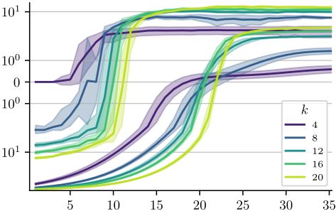
small values. The periodic schedules achieve significantly higher scores consistently, and their quality improves together with the quality of the initial RFM. Interestingly, the maxima are attained much earlier (around step 15). This shows that a slight initial improvement of the RFM schedule leads to a significant boost of a sampled periodic schedule.
A more detailed analysis is in the extended version of this paper [Klaˇska et al., 2023, App. A]. We mention that the periodic schedules are typically 100-200 nodes long with traverse time exceeding 12 working shifts. All RFMs were optimized with memory size 1, which explains their lower values. Experiments with larger memory are also in [Klaˇska et al., 2023, App. A]. In conclusion, to find periodic schedules as RFM, the memory has to be large (to encode, say, 200 long cycle on 4k + 1 nodes), which is expensive for larger graphs. Smaller memories above 1 do not help significantly. Therefore optimizing memoryless RFM combined with determinization gives satisfactorily high values with low runtimes.
7 Conclusion
We introduced the infinite horizon recurrent routing problem (IHRRP) and presented two solution concepts: randomized finite memory (RFM) and periodic schedules. We proved that even the problem of bounding the value of an optimal periodic schedule is PSPACE-hard. Then, we proposed an algorithmic solution based on randomized algorithms. We apply differentiable programming with optimization techniques to synthesize promising RFM schedules that, by random sampling procedure, yield strong periodic schedules. We demonstrated on reasonably-sized examples that our approach stably produces long schedules that achieve a high mean payoff.
Acknowledgments
This work has been supported by the Czech Science Foundation, Grant No. 21-24711S.
@inproceedings{ijcai2023p598,
  title     = {Mean Payoff Optimization for Systems of Periodic Service and Maintenance},
  author    = {Klaska, David and Kucera, Antonin and Musil, Vit and Rehak, Vojtech},
  booktitle = {Proceedings of the Thirty-Second International Joint Conference on
               Artificial Intelligence, {IJCAI-23}},
  publisher = {International Joint Conferences on Artificial Intelligence Organization},
  editor    = {Edith Elkind},
  pages     = {5386--5393},
  year      = {2023},
  month     = {8},
  note      = {Main Track},
  doi       = {10.24963/ijcai.2023/598},
  url       = {https://doi.org/10.24963/ijcai.2023/598},
}
TY - CPAPER TI - Mean Payoff Optimization for Systems of Periodic Service and Maintenance AU - Klaska, David AU - Kucera, Antonin AU - Musil, Vit AU - Rehak, Vojtech T2 - Proceedings of the Thirty-Second International Joint Conference on Artificial Intelligence, IJCAI-23 PB - International Joint Conferences on Artificial Intelligence Organization PY - 2023 SP - 5386 EP - 5393 DO - 10.24963/ijcai.2023/598 UR - https://doi.org/10.24963/ijcai.2023/598 ER -Copied
Machine-readable versions of this paper, for tools and AI agents:





